Green-Naghdi-Rivlin (GNR) theorem

We will now study a central theorem in continuum mechanics that illustrates how the principle of (Euclidean) relativity in conjunction with the laws of thermodnamics yields all the balance principles of continuum mechanics. To understand this, we first need to understand the notion of objectivity of tensor fields. In the process of proving the Green-Naghdi-Rivlin theorem, we will also introduce the crucial notion of the stress tensor.

Observer transformations

Recall from our discussion of kinematics that an observer is characterized by a map that assigns to each event in spacetime a unique coordinate in $\mathbb{R}^3\times\mathbb{R}$. If two different observers, $\mathcal{O}$ and $\mathcal{O}^+$, assign coordinates $\mathsf{x},t$ and $\mathsf{x}^+,t^+$, respectively, for the same event, then the map $$(\mathsf{x},t) \in \mathbb{R}^3\times\mathbb{R} \to (\mathsf{x}^+,t^+) \in \mathbb{R}^3\times\mathbb{R}$$ is called an observer transformation. Note that an observer transformation is a diffeomorphism of spacetime. This means that the map displayed above is continuously differentiable, and invertible, with the inverse also being continuously differentiable.

Remark

The reason for using the notation $(\mathsf{x}^+,t^+)$ for the space and time coordinates for the second observer is simply to emphasize that we will shortly focus on a special class of observer transformations that can alternatively also be interpreted as a superimposed rigid body motion.

Let us now focus on a special class of observer transformations, namely those that preserve the distance between two points in space, and the time interval between two events. To make this concrete, suppose that we consider two events, which have spacetime coordinates $(\mathsf{x}_1,t_1)$ and $(\mathsf{x}_2,t_2)$ according to observer $\mathcal{O}$. Let the space and time coordinates of the same event with respect to another observer $\mathcal{O}^+$ be $(\mathsf{x}_2^+,t_2^+)$. The requirement that the two observers measure the same distance between these two points and record the same time interval between these two events can be expressed using the following equations: $$\begin{split} \lVert \mathsf{x}_1 - \mathsf{x}_2 \rVert &= \lVert \mathsf{x}_1^+ - \mathsf{x}_2^+ \rVert,\\ t_1 - t_2 &= t_1^+ - t_2^+. \end{split}$$ A general class of observer transformations that satisfies this requirement can be written as $$\begin{split} \mathsf{x}^+(\mathsf{x},t) &= \mathsf{c}(t) + \mathsf{Q}(t)(\mathsf{x} - \mathsf{x}_0),\\ t^+(\mathsf{x},t) &= t, \end{split}$$ as can be easily verified. Here, $\mathsf{c}(t) \in \mathbb{R}^3$, $\mathsf{x}_0 \in \mathbb{R}^3$, and $\mathsf{Q}(t) \in SO(3)$ for every $t \in \mathbb{R}$. For the sake of notational succinctness, we will write $\mathsf{x}^+$ and $\mathsf{t}^+$ for $\mathsf{x}^+(\mathsf{x},t)$ and $t^+(\mathsf{x},t)$, respectively. Observer transformations of this form are called Euclidean transformations. In the special case when we insist that $\mathsf{c}(t) = \mathsf{c}_0t$ for some constant vector $\mathsf{c}_0 \in \mathbb{R}^3$, and $\mathsf{Q}(t) = \mathsf{Q}_0$ for some constant $\mathsf{Q}_0 \in SO(3)$, these observer transformations are called Galilean transformations.

Remark

In special relativity, one considers observers who agree upon the proper time interval between two events. Given two events with coordinates $(\mathsf{x}_1,t_1)$ and $(\mathsf{x}_2,t_2)$ according to an observer, the proper time interval between these two events is defined as $$\Delta \tau = c^2(t_1 - t_2)^2 - \lVert \mathsf{x}_1 - \mathsf{x}_2\rVert^2.$$ Here, $c \in \mathbb{R}$ stands for the velocity of light in vacuum. In special relativity, two consenting observers agree only upon the proper time interval. Notice that this does not require them to agree upon distances between two points in space, or the time time interval between two events, in sharp constrast to classical (Newtonian) physics.

Galilean transformations are used in the classical principle of relativity: the laws of classical physics remain invariant with respect to Galilean transformations. In continuum mechanics, we will postulate the invariance of the continuum analogues of the first and second laws of thermodynamics with respect to Euclidean transformations. This is the key idea behind the Green-Naghdi-Rivlin theorem.

Objectivity

We will now introduce a crucial concept called objectivity for scalar, vector and tensor fields. Throughout this discussion we will assume that we have two observers $\mathcal{O}$ and $\mathcal{O}^+$ who are related to each other according to a Euclidean transformation. We will use the same convention to denote space and time coordinates of an event according to these observers as in the previous section.

Scalar fields

Let us start with the simple case of a scalar field $f:\mathbb{R}^3 \times \mathbb{R} \to \mathbb{R}$, as measured by the observer $\mathcal{O}$. Let us denote the same scalar field, as measured by the observer $\mathcal{O}^+$, as $f^+:\mathbb{R}^3\times\mathbb{R} \to \mathbb{R}$. The scalar field is said to be objective if $$f(\mathsf{x},t) = f^+(\mathsf{x}^+,t^+).$$ To better appreciate the notion of objectivity, consider the temperature field $\hat{\Theta}_t:\mathcal{B} \to \mathbb{R}$ of a continuum body $\mathcal{B}$ at the current time instant $t$. As measured by the observer $\mathcal{O}$, the temperature at $\mathsf{x} \in B_t$ can be written as $\theta(\mathsf{x},t)$. With respect to the observer $\mathcal{O}^+$, the temperature of the point $\mathsf{x}^+(\mathsf{x},t) \in B_t^+$ is given by $\theta^+(\mathsf{x}^+,t^+)$. It is evident that both these observers measure the same value of the temperature at the same material point. Equivalently, we see that the temperature field is objective.

Vector fields

The spacetime diffeomorphism characterizing an observer transformation naturally induces a basis at each tangent space to $\mathbb{R}^3$. Let $(\mathsf{e}_i)$ be a basis to the tangent space at $\mathsf{x} \in \mathbb{R}^3$, according to the observer $\mathcal{O}$. The corresponding basis $(\mathsf{e}_i^+)$ of the tangent space $T_{\mathsf{x}^+}\mathbb{R}^3$ according to the observer $\mathcal{O}^+$ can be computed as follows: $$\mathsf{e}_i^+(\mathsf{x}^+,t^+) = \nabla \mathsf{x}^+(\mathsf{x},t) \cdot \mathsf{e}_i = \mathsf{Q}(t)\mathsf{e}_i.$$

Remark

Note that $\mathsf{Q}(t):T_{\mathsf{x}}\mathbb{R}^3 \to T_{\mathsf{x}^+}\mathbb{R}^3$, and can be written as $$Q(t) = \sum \mathsf{e}_i^+(\mathsf{x}^+,t^+) \otimes \mathsf{e}_i.$$ It is easy to verify the orthogonality of $Q(t)$ directly using this expression. Note that a similar expression applies for $\mathsf{Q}^T(t):T_{\mathsf{x}^+}\mathbb{R}^3 \to T_{\mathsf{x}}\mathbb{R}^3$.

A vector field $\mathsf{w}$ on $\mathbb{R}^3$ is said to be objective if $$\mathsf{w}^+(\mathsf{x}^+,t^+) = \mathsf{Q}(t)\mathsf{w}(\mathsf{x},t).$$ To understand what this means, let us compute the local representation of the vector field according to both observers. According to $\mathcal{O}$, let $$\mathsf{w}(\mathsf{x},t) = \sum w_i(\mathsf{x},t)\mathsf{e}_i.$$ If $\mathsf{w}$ is an objective vector field, then its representation with respect to $\mathcal{O}^+$ is computed as $$\begin{split} \mathsf{w}^+(\mathsf{x}^+,t^+) &= \mathsf{Q}(t)\left(\sum w_i(\mathsf{x},t) \mathsf{e}_i\right)\\ &= \sum w_i(\mathsf{x},t) \mathsf{Q}(t)\mathsf{e}_i\\ &= \sum w_i(\mathsf{x},t) \mathsf{e}_i^+(\mathsf{x}^+,t^+). \end{split}$$ Comparing this with the coordinate representation $$\mathsf{w}^+(\mathsf{x}^+,t^+) = \sum w_i^+(\mathsf{x}^+,t^+) \mathsf{e}_i^+(\mathsf{x}^+,t^+)$$ of the vector field according to the observer $\mathcal{O}^+$, we see that, for $i = 1,2,3$, $$w_i^+(\mathsf{x}^+,t^+) = w_i(\mathsf{x},t).$$ In other words, the components fields of an objective vector field are objective scalar fields. The physical intuition behind this is that if a vector field is objective, then a Euclidean transformation just rotates the basis vectors of each tangent space uniformly, but doesn't affect the components of an objective vector field with respect to these bases. In other words, an objective vector field rotates along with the observer globally.

Tensor fields

The objectivity of tensor fields is defined in a manner analogous to that of vector fields. If $\mathsf{A}$ is a tensor field of order $k$ on $\mathbb{R}^3$, its component representation according to observer $\mathcal{O}$ can be written as $$\mathsf{A}(\mathsf{x},t) = \sum A_{i_1\ldots i_k}(\mathsf{x},t) \, \mathsf{e}_{i_1} \otimes \ldots \otimes \mathsf{e}_{i_k}.$$ The tensor field $\mathsf{A}$ is said to be objective if, according to the observer $\mathcal{O}^+$ who is related to the observer $\mathcal{O}$ by a Euclidean transformation, the tensor field admits the representation $$\mathsf{A}^+(\mathsf{x}^+,t^+) = \sum A_{i_1\ldots i_k}(\mathsf{x},t) \, \mathsf{e}_{i_1}^+(\mathsf{x}^+,t^+) \otimes \ldots \otimes \mathsf{e}_{i_k}^+(\mathsf{x}^+,t^+).$$ There are many equivalent ways of expressing this. For instance, the foregoing equation can be written as $$\mathsf{A}^+(\mathsf{x}^+,t^+) = \sum A_{i_1\ldots i_k}(\mathsf{x},t) \, \mathsf{Q}(t)\mathsf{e}_{i_1} \otimes \ldots \otimes \mathsf{Q}(t) \mathsf{e}_{i_k}.$$ In terms of the components of the tensor fields, we can express the condition for objectivity as $$A_{i_1\ldots i_k}^+(\mathsf{x}^+,t^+) = A_{i_1\ldots i_k}(\mathsf{x},t).$$ An analogous interpretation of the objectivity of tensor fields as in the case of vector fields should be evident.

Owing to its practical utility, it is useful to consider the special case of a second order tensor field. In this case, the objectivity condition for a second order tensor field $\mathsf{A}$ can be expressed compactly as follows: $$\mathsf{A}^+(\mathsf{x}^+,t^+) = \mathsf{Q}(t)\mathsf{A}(\mathsf{x},t)\mathsf{Q}^T(\mathsf{x}^+,t^+).$$ This can be easily verified by an explicit computation, and is left as a simple exercise. This form of the objectivity condition for second order tensors will be used extensively in the sequel.

Remark

To keep the notation manageable, we will often drop the arguments and write the objectivity condition for a second order tensor field as just $\mathsf{A}^+ = \mathsf{Q}\mathsf{A}\mathsf{Q}^T$.

Objectivity of continuum fields

As should be clear now, we would ideally like the various scalar, vector and tensor fields that enter a continuum description of the first and second laws of thermodynamics need to be objective. The reason is that this enforces observer invariance of the various continuum fields involved. Let us now make this notion formally precise. As before, we will be dealing with two observers $\mathcal{O}$ and $\mathcal{O}^+$ who are related according to a Euclidean transformation.

To begin with, we will postulate that all the scalar fields involved in the first and second laws of thermodynamics are objective. To be specific, we postulate the following relations: $$\begin{split} \rho^+(\mathsf{x}^+,t^+) &= \rho(\mathsf{x},t),\\ e^+(\mathsf{x}^+,t^+) &= e(\mathsf{x},t),\\ r^+(\mathsf{x}^+,t^+) &= r(\mathsf{x},t),\\ \eta^+(\mathsf{x}^+,t^+) &= \eta(\mathsf{x},t),\\ \theta^+(\mathsf{x}^+,t^+) &= \theta(\mathsf{x},t),\\ h^+(\mathsf{x}^+,t^+,\mathsf{n}^+(\mathsf{x}^+,t^+)) &= h(\mathsf{x},t,\mathsf{n}(\mathsf{x},t)). \end{split}$$ Notice how the unit normal figures in the last expression. Since a unit normal is an element of the appropriate tangent space, it transforms objectively: $\mathsf{n}^+(\mathsf{x}^+,t^+) = \mathsf{Q}(t)\mathsf{n}(\mathsf{x},t)$.

Let us now turn to the various vector fields that figure in the first law of thermodynamics. To start with, consider the simple case of a particle moving in three dimensional space such that at time $t \in I \subseteq \mathbb{R}$, the particle occupies position $\mathsf{x}(t)\in\mathbb{R}^3$, according to observer $\mathcal{O}$. The velocity and acceleration of this particle, as observed by $\mathcal{O}$ are given by $\dot{\mathsf{x}}(t) = d\mathsf{x}(t)/dt$ and $\ddot{\mathsf{x}}(t) = d^2\mathsf{x}(t)/dt^2$, respectively. Let us now compute how the motion of the same particle according to an observer $\mathcal{O}^+$ who is related to $\mathcal{O}$ by a general Euclidean transformation, $$\mathsf{x}^+(\mathsf{x},t) = \mathsf{c}(t) + \mathsf{Q}(t)\mathsf{x}, \qquad t^+ = t,$$ looks like. The position, velocity and acceleration of the same particle as observed by $\mathcal{O}^+$ can be easily computed as $$\begin{split} \mathsf{x}^+(t) &= \mathsf{c}(t) + \mathsf{Q}(t)\mathsf{x}(t),\\ \mathsf{v}^+(t) &= \dot{\mathsf{c}}(t) + \dot{\mathsf{Q}}(t)\mathsf{x}(t) + \mathsf{Q}(t)\mathsf{v}(t),\\ \mathsf{a}^+(t) &= \ddot{\mathsf{c}}(t) + \ddot{\mathsf{Q}}(t)\mathsf{x}(t) + 2\dot{\mathsf{Q}}(t)\mathsf{v}(t) + \mathsf{Q}(t)\mathsf{a}(t). \end{split}$$

Remark

Notice the close similarity between the first equation in the list of three equations above, and the Euclidean transformation relation observers $\mathcal{O}$ and $\mathcal{O}^+$. In the former, $\mathsf{x}(t)$ is a time dependent trajectory of a particle in three dimensional space. In the latter, $\mathsf{x}$ stands for a generic point in space, and has no time dependence at all. The meaning of equations like these should always be inferred carefully from the appropriate context.

Note that neither the velocity, nor the acceleration of the particle, are objective vector fields in general. In the special case of a Galilean transformation, howevever, when $\mathsf{c}(t) = \mathsf{c}_0 t$ for some constant $\mathsf{c}_0 \in \mathbb{R}^3$, and when $\mathsf{Q}(t) = \mathsf{Q}_0$ for some constant rotation map $\mathsf{Q}_0 \in SO(3)$, we see that $$\begin{split} \mathsf{v}^+(t) &= \mathsf{c}_0 + \mathsf{Q}_0\mathsf{v}(t),\\ \mathsf{a}^+(t) &= \mathsf{Q}_0\mathsf{a}(t). \end{split}$$ We thus see that the velocity vector is still not objective, but the acceleration is in fact an objective vector. This is the familiar result in elementary classical physics that if two observers are moving relative to each other with a constant velocity, then they will measure the same acceleration of any moving body they observe, but disagree on the velocity.

Let us now move on to the other vector fields appearing in the first law of thermodynamics. Let us look at the surface traction first. Recall that the traction vector was introducted to model the surface force on a continuum. Thus, given any small areal $\Delta a$ centered at $\mathsf{x} \in \partial B_t$ with normal $\mathsf{n}(\mathsf{x},t)$, we modeled the force acting on this small area as $\mathsf{t}(\mathsf{x},t,\mathsf{n}(\mathsf{x},t))\Delta a$. We will now extend the traction defined on the surface $\partial B_t$ to the whole of $B_t$ so that given any $\mathsf{x} \in B_t$ and $\mathsf{n} \in T_{\mathsf{x}}B_t$, we have uniquely defined vector $\mathsf{t}(\mathsf{x},t,\mathsf{n}) \in T_{\mathsf{x}}B_t$. The idea behind this extension is that we can compute a force on every infinitesimal area at every point in the continuum, as shown in the following figure:

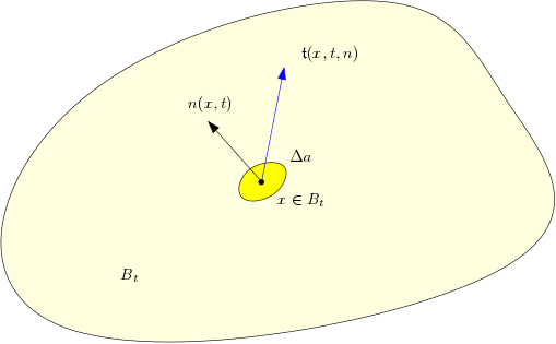
We will take it as a basic postulate of continuum mechanics that this extension is always well-defined. The simplest means to appreciate this postulate is by going back to the spring mass analogy given earlier - any force applied on the surface atoms percolates to the interior as a consequence of the collective response of all the springs to the applied force.

We are now in a position to state an important postulate: we will henceforth consider the traction vector field as being objective. This means that if two observers $\mathcal{O}$ and $\mathcal{O}^+$ who are related by a Euclidean transformation observe the same process, then $$\mathsf{t}^+(\mathsf{x}^+,t^+,\mathsf{n}^+(\mathsf{x}^+,t^+)) = \mathsf{Q}(t) \mathsf{t}(\mathsf{x},t,\mathsf{n}(\mathsf{x},t)).$$ To understand the rationale behind the postulate concerning the objectivity of the traction vector field, note that the traction vector represents the internal response of the continuum due to externally applied forces and energy supplied in the form of heat. Thus the postulate that the traction vector field is objective simply means that this internal response of the continuum is independent of observer transformations.

Remark

Another way of rationalizing this is to note that when viewed from the atomistic viewpoint, the energy of a collection of atoms, called an interatomic potential, can only depend on the relative positions of the atoms, and not on their absolute positions, if the energy is to describe a physically realistic internal energy that is invariant with respect to translations and rotations. Since Euclidean transformations do not change the relative positions of the atoms, it makes sense to postulate that the traction vector field is objective. Note that the need to make this a postulate is simply because the continuum is a mathematical construct, and the behavior of dynamical fields defined on the continuum need to be postulated based on the behavior of their true atomistic counterparts.

Finally, let us turn to the body force density. Rather than talk about the body force density $\mathsf{b}$ directly, we will consider instead the quantity $\mathsf{b} - \mathsf{a}$, and postulate that this quantity is objective. Thus, from the point of view of two observers $\mathcal{O}$ and $\mathcal{O}^+$ who are related by a Euclidean transformation, we postulate that $$\mathsf{b}^+(\mathsf{x}^+,t^+) - \mathsf{a}^+(\mathsf{x}^+,t^+) = \mathsf{Q}(t)(\mathsf{b}(\mathsf{x},t) - \mathsf{a}(\mathsf{x},t)).$$ Recall that we studied the transformation rules for the spatial accleration (which is not an objective vector field) earlier. Using that in conjunction with the equation presented above gives the observer transformation rule for the body force density.

To understand the idea behind this postulate, it is helpful to consider a very simple system of a mass connected by a spring to a stationary point. Assuming the spring to be linear with a spring constant $k$, the equation governing the dynamics of the mass when subject to a force $mb$, according to observer $\mathcal{O}$, is given by $$mb - k(x - x_0) = ma.$$ Here, $\mathsf{x}_0$ is the coordinate of the fixed point to which the spring is attached. The same equation takes the following form according to an observer $\mathcal{O}^+$ who is related to $\mathcal{O}$ by a Euclidean transformation: $$mb^+ - k(x^+ - x_0^+) = ma^+.$$ Using the fact that $x^+ - x_0^+ = \mathsf{Q}(t)(x - x_0)$, it is easy to see that $$b^+ - a^+ = Q(b - a).$$ This is just the transformation rule postulated earlier. While this does not prove the postulate (which is why it is a postulate in the first place), it provides a simple means to appreciate why the postulate is formulated in its specific form.

Observer invariance of the second law of thermodynamics

We have now all the necessary tools to study the consequences of requiring that the first and second laws of thermodynamics are invariant with respect to Euclidean observer transformations. We will start with the second law of thermodynamics since it is much easier to deal with.

Let $\mathcal{O}$ and $\mathcal{O}^+$ be two observers who are related by a Euclidean transformation. Let us write the second law according to the observer $\mathcal{O}^+$: $$\frac{d}{dt^+}\int_{B_t^+} \rho^+(\mathsf{x}^+,t^+) \, dv^+ \ge \int_{B_t^+} \frac{\rho^+(\mathsf{x}^+,t^+)r^+(\mathsf{x}^+,t^+)}{\theta^+(\mathsf{x}^+,t^+)} \, dv^+ - \int_{\partial B_t^+} \frac{h^+(\mathsf{x}^+,t^+,\mathsf{n}^+(\mathsf{x}^+,t^+))}{\theta^+(\mathsf{x}^+,t^+)}\,da^+.$$ Let us now change the variables from $(\mathsf{x}^+,t^+)$ to $(\mathsf{x},t)$. Since the second law involves only scalar fields, each of which is objective, the transformation of the integrands is trivial. The volume and area integrals transform according to the usual change of variables rules that we studied earlier. Specifically, note that for any scalar field $f:B_t \to \mathbb{R}$, $$\begin{split} \int_{B_t^+} f^+(\mathsf{x}^+,t^+)\eta^+(\mathsf{x}^+,t^+)\,dv^+ &= \int_{B_t} f(\mathsf{x},t) \text{det}(\mathsf{Q}(t))\,dv\\ &= \int_{B_t} f(\mathsf{x},t)\,dv. \end{split}$$ In deriving the last expression, we used the fact that $\mathsf{Q}(t)$ is orthogonal.

To understand how area integrals transform, let us revisit the change of area formula in the case of a Euclidean observer transformation: $$\mathsf{n}^+(\mathsf{x}^+,t^+)\Delta a^+ = \text{det}(\mathsf{Q}(t))\mathsf{Q}^{-T}\mathsf{n}(\mathsf{x},t)\Delta a.$$ Noting that $\mathsf{Q}^{-T}(t) = \mathsf{Q}(t)$ and that $\mathsf{n}^+ = \mathsf{Q}\mathsf{n}$, it follows that $\Delta a^+ = \Delta a$. We can thus transform the area integral of a scalar field $g:B_t \to \mathbb{R}$ as: $$\int_{\partial B_t^+} g^+(\mathsf{x}^+,t^+)\,da^+ = \int_{\partial B_t} g(\mathsf{x},t)\,da.$$

Putting all this together, we can transform the second law as observed by the observer $\mathcal{O}^+$ as $$\frac{d}{dt}\int_{B_t} \rho(\mathsf{x},t)\eta(\mathsf{x},t)\,dv \ge \int_{B_t} \frac{\rho(\mathsf{x},t)r(\mathsf{x},t)}{\theta(\mathsf{x},t)}\,dv - \int_{B_t} \frac{h(\mathsf{x},t,\mathsf{n}(\mathsf{x},t))}{\theta(\mathsf{x},t)}\,da.$$ But this is precisely the second law as recorded by the observer $\mathcal{O}$. We thus see that the second law of thermodynamics is naturally invariant with respect to Euclidean observer transformations. In other words, there are no additional restrictions on the various scalar fields in the second law as a consequence of Euclidean observer invariance.

Observer invariance of the first law of thermodynamics

Unlike the second law of thermodynamics, we will see shortly that requiring the first law to be invariant with respect to Euclidean observer transformations yields very important and new information regarding the various continuum fields. In particular, we will see that the principles of conservation of mass, linear momentum and angular momentum, all follow from this basic invariance requirement. This remarkable result is known as the Green-Naghdi-Rivlin theorem. We will develop this in two stages: we will first study the consequences of requiring the first laws to be invariant with respect to observers who are moving relative to each other with a constant velocity, and subsequently with respect to observers who are rotating with respect to each other.

Mass and linear momentum balance

Let us first consider the case when the observers $\mathcal{O}$ and $\mathcal{O}^+$ are related to each other according to the following transformation: $$\mathsf{x}^+ = \mathsf{x} + \mathsf{c}_0 t, \quad t^+ = t.$$ Here $\mathsf{c}_0\in\mathbb{R}^3$ is a constant vector. Note that this is the constant velocity with which the two observers are moving relative to each other. Note also that $\mathsf{Q}(t) = \mathsf{I}$ in this case.

Let us write the first law of thermodynamics according to the observer $\mathcal{O}^+$: $$\begin{split} \frac{d}{dt^+}\int_{B_t^+} \rho^+\left(e^+ + \frac{1}{2}\mathsf{v}^+\cdot\mathsf{v}^+\right)\,dv^+ &= \int_{B_t^+} \rho^+ \mathsf{b}^+\cdot\mathsf{v}^+\,dv^+ + \int_{\partial B_t^+} \mathsf{t}^+\cdot\mathsf{v}^+\,da^+\\ & + \int_{B_t^+} \rho^+r^+\,dv^+ - \int_{\partial B_t^+} h^+\,da^+. \end{split}$$ Note that we have dropped all the arguments in the equation above to keep the notation manageable. Let us now transform the coordinates from $(\mathsf{x}^+,t^+)$ to $(\mathsf{x},t)$. Using the transformation rules derived earlier, we seee that all the scalar fields remain invariant, and the vector fields involved transform as follows: $$\begin{split} \mathsf{v}^+ &= \mathsf{v} + \mathsf{c}_0,\\ \mathsf{a}^+ &= \mathsf{a},\\ \mathsf{b}^+ &= \mathsf{b},\\ \mathsf{t}^+ &= \mathsf{t}. \end{split}$$ Using this, we can write the first law as follows: $$\begin{split} \frac{d}{dt}\int_{B_t} \rho\left(e + \frac{1}{2}((\mathsf{v} + \mathsf{c}_0)\cdot(\mathsf{v} + \mathsf{c}_0)\right)dv &= \int_{B_t} \rho \mathsf{b} \cdot (\mathsf{v} + \mathsf{c}_0) \, dv\\ & + \int_{\partial B_t} \mathsf{t} \cdot (\mathsf{v} + \mathsf{c}_0)\, da\\ & + \int_{B_t} \rho r \,dv - \int_{\partial B_t} h\,da. \end{split}$$ Let us now consider the first law of thermodynamics according to the observer $\mathcal{O}$: $$\frac{d}{dt}\int_{B_t} \rho\left(e + \frac{1}{2}\mathsf{v}\cdot\mathsf{v}\right)\,dv = \int_{B_t} \rho\mathsf{b}\cdot\mathsf{v}\,dv + \int_{\partial B_t}\mathsf{t}\cdot\mathsf{v}\,da + \int_{B_t} \rho r \, dv - \int_{\partial B_t} h\,da.$$ Since this equation and the transformed equation of the first law according to the observer $\mathcal{O}^+$ that we presented earlier, we immediately get the following equation: $$\frac{d}{dt}\int_{B_t} \rho\left(\mathsf{v}\cdot\mathsf{c}_0 + \frac{1}{2}\mathsf{c}_0\cdot\mathsf{c}_0\right)dv = \int_{B_t} \mathsf{b}\cdot\mathsf{c}_0\,dv + \int_{\partial B_t} \mathsf{t}\cdot\mathsf{c}_0\,da.$$ Since this equation is true for arbitrary $\mathsf{c}_0 \in \mathbb{R}^3$, writing the same equation for $-\mathsf{c}_0$ and adding the two equations, we get $$\frac{1}{2}\mathsf{c}_0\cdot\mathsf{c}_0\frac{d}{dt}\int_{B_t} \rho\,dv = 0 \quad\Rightarrow\quad \frac{d}{dt}\int_{B_t} \rho(\mathsf{x},t)\,dv = 0.$$ We thus see that the total mass contained in the region $B_t$ is conserved. But this is precisely the law of conservation of mass. Taking the time derivative inside the integral, we see that $$\int_{B_t} \left(\frac{D\rho}{Dt} + \rho\,\text{div }\mathsf{v}\right) = 0.$$ Using the localization lemma, we get the familiar mass continuity equation $$\frac{D\rho(\mathsf{x},t)}{Dt} + \rho(\mathsf{x},t)\,\text{div }\mathsf{v}(\mathsf{x},t) = 0.$$ Notice how the simple requirement that the first law of thermodynamics is invariant with respect to observers moving relative to each other with a constant velocity has already yielded the mass conservation equation!

We're not done yet. Using the mass continuity equation in conjunction with the Reynolds' transport theorem, we see that, for any arbitray $\mathsf{c}_0 \in \mathbb{R}^3$, $$\int_{B_t} \rho \frac{D\mathsf{v}}{Dt}\cdot\mathsf{c}_0\,dv = \int_{B_t} \mathsf{b}\cdot\mathsf{c}_0\,dv + \int_{\partial B_t} \mathsf{t}\cdot\mathsf{c}_0\,da.$$ Note that we cannot directly localize this integral equation on account of the surface integral. Let us now look into this; in the process we will develop a crucial notion in continuum mechanics, that of the stress tensor. The kernel of the surface term $\mathsf{t}(\mathsf{x},t,\mathsf{n}(\mathsf{x},t))\cdot\mathsf{c}_0$ is a function of $\mathsf{x},t,\mathsf{n}$. The Cauchy localization lemma immediately implies the existence of a vector field $\mathsf{t}_{\mathsf{c}_0}$ on $B_t$ such that $$\mathsf{t}(\mathsf{x},t,\mathsf{n}(\mathsf{x},t))\cdot\mathsf{c}_0 = \mathsf{t}_{\mathsf{c}_0}(\mathsf{x},t)\cdot\mathsf{n}(\mathsf{x},t),$$ for every $\mathsf{c}_0 \in \mathbb{R}^3$. To understand how the vector field $\mathsf{t}_{\mathsf{c}_0}$ depends on $\mathsf{c}_0$, consider any arbitrary $\mathsf{c}_0,\mathsf{c}_1 \in \mathbb{R}^3$ and $a \in \mathbb{R}$, and note that $$\begin{split} \mathsf{t}_{\mathsf{c}_0 + a\mathsf{c}_1}(\mathsf{x},t)\cdot\mathsf{n}(\mathsf{x},t) &= \mathsf{t}(\mathsf{x},t,\mathsf{n}(\mathsf{x},t))\cdot(\mathsf{c}_0 + a\mathsf{c}_1)\\ &= \mathsf{t}(\mathsf{x},t,\mathsf{n}(\mathsf{x},t))\cdot\mathsf{c}_0 + a \mathsf{t}(\mathsf{x},t,\mathsf{n}(\mathsf{x},t))\cdot\mathsf{c}_1\\ &= \mathsf{t}_{\mathsf{c}_0}(\mathsf{x},t)\cdot\mathsf{n}(\mathsf{x},t) + a\mathsf{t}_{\mathsf{c}_1}(\mathsf{x},t)\cdot\mathsf{n}(\mathsf{x},t). \end{split}$$ We thus see that $\mathcal{t}_{\mathsf{c}_0}$ is a linear function of $\mathsf{c}_0$. This implies that there exists a linear map $\sigma(\mathsf{x}, t):T_{\mathsf{x}}B_t \to T_{\mathsf{x}}B_t$ such that $$\mathsf{t}_{\mathsf{c}_0}(\mathsf{x},t) = \sigma^T(\mathsf{x},t)\mathsf{c}_0.$$

Remark

Note that if $\sigma$ is a linear map, so is $\sigma^T$. The reason for using the transpose of $\sigma$ in the equation $\mathsf{t}_{\mathsf{c}_0}(\mathsf{x},t) = \sigma^T(\mathsf{x},t)\mathsf{c}_0$ is primarily a matter of convention so that the components of $\sigma$ with respect to a chosen basis has the familiar interpretation used in engineering.

Remark

Note that the Cauchy localization lemma only shows the existence of a linear map of the form $\sigma(\mathsf{x},t):T_{\mathsf{x}}\mathbb{R}^3 \to T_{\mathsf{x}}\mathbb{R}^3$. However, in our case, since $B_t$ is an open subset of $\mathbb{R}^3$, we have the natural identity $T_{\mathsf{x}}B_t \equiv T_{\mathsf{x}}\mathbb{R}^3$. The reason for preferring $T_{\mathsf{x}}B_t$ over $T_{\mathsf{x}}\mathbb{R}^3$ will become evident soon.

The linear map, or equivalently, the second order tensor, $\sigma(\mathsf{x},t)$ is called the Cauchy stress tensor. With this definition, we see that for every $\mathsf{c},\mathsf{n} \in T_{\mathsf{x}}B_t$, $$\mathsf{t}(\mathsf{x},t,\mathsf{n})\cdot\mathsf{c} = \sigma^T(\mathsf{x},t)\mathsf{c} \cdot \mathsf{n} = \mathsf{c} \cdot \sigma(\mathsf{x},t)\mathsf{n}.$$ Since this is true for every $\mathsf{c} \in T_{\mathsf{x}}B_t$, we obtain the following expression relating the traction vector and the Cauchy stress tensor: $$\mathsf{t}(\mathsf{x},t,\mathsf{n}) = \sigma(\mathsf{x},t)\mathsf{n}.$$ This equation tells us that the Cauchy stress tensor allows us to compute the surface force acting on any infinitesimal area with a prescribed unit normal.

To understand what the Cauchy stress tensor means, let us consider the component representation of the equation $\mathsf{t}(\mathsf{x},t,\mathsf{n}) = \sigma(\mathsf{x},t)\mathsf{n}$ with respect to an orthonormal basis $(\mathsf{e}_i)$ of $T_{\mathsf{x}}B_t$: $$t_i(\mathsf{x},t,\mathsf{n}) = \sum \sigma_{ij}(\mathsf{x},t) n_j,$$ where $$\sigma(\mathsf{x},t) = \sum \sigma_{ij}(\mathsf{x},t) \mathsf{e}_i \otimes \mathsf{e}_j$$ is the coordinate representation of the Cauchy stress tensor. To physically interpret the components of the Cauchy stress tensor, consider a cube with one of its vertices at $\mathsf{x}\in B_t$ as shown below:

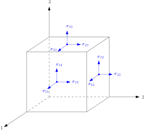
We thus see that $\sigma_{ij}(\mathsf{x},t)$ represents the force along the $i^{\text{th}}$ coordinate axis on an infinitesimal area element at $\mathsf{x} \in B_t$ whose normal is along the $j^{\text{th}}$ coordinate axis.

Returning back to our discussion of the invariance of the first law of thermodynamics with respect to Euclidean observer transformations, let us use the Cauchy stress tensor to localize the equation $$\int_{B_t} \rho \frac{D\mathsf{v}}{Dt}\cdot\mathsf{c}_0\,dv = \int_{B_t} \mathsf{b}\cdot\mathsf{c}_0\,dv + \int_{\partial B_t} \mathsf{t}\cdot\mathsf{c}_0\,da.$$ Using the fact that $\mathsf{t} = \sigma\mathsf{n}$ and using the divergence theorem, we see that $$\begin{split} \int_{\partial B_t} \mathsf{t}\cdot\mathsf{c}_0 \,da &= \int_{\partial B_t} \mathsf{c}_0 \cdot \sigma \mathsf{n}\,da\\ &= \int_{B_t} \text{div}(\mathsf{c}_0\cdot\sigma)\,dv. \end{split}$$ Using this result, and the fact that $\mathsf{c}_0$ is a constant vector, we obtain the following integral relation: $$\int_{B_t} \left(\rho\frac{D\mathsf{v}}{Dt} - \mathsf{b} - \text{div }\sigma\right)\cdot\mathsf{c}_0\,dv = 0.$$ The localization lemma immediately yields the following differential equation: $$\rho(\mathsf{x},t)\frac{D\mathsf{v}(\mathsf{x},t)}{Dt} = \mathsf{b}(\mathsf{x},t) + \text{div }\sigma(\mathsf{x},t).$$ This equation is the continuum analogue of Newton's second laws $ma = F$, and is hence called the linear momentum balance equation. The means to understand this physically is as follows. As a consequence of the application of external forces (both body forces and surface tractions), the continuum responds by generating generalized internal forces, which we have modeled using the Cauchy stress tensor. The term $\mathsf{b}(\mathsf{x},t) + \text{div }\sigma(\mathsf{x},t)$ thus represents the net force acting at an interior point $\mathsf{x}\in B_t$. This net force is equal to its acceleration $\rho(\mathsf{x},t)\mathsf{a}(\mathsf{x},t)$.

We have thus obtained both the balance of mass and balance of linear momentum from the first law of thermodynamics by merely insisting that the first law is invariant with respect to two observers who are in relative motion with respect to each other with a constant velocity!

Angular momentum balance

In the previous section, we obtained both the mass and linear momentum conservation equations as a consequence of the invariance of the first law of thermodynamics with respect to Euclidean transformations characterized by a constant velocity relative motion of the observers. Let us now consider the consequences of the first law being invariant with respect to observers $\mathcal{O}, \mathcal{O}^+$ whose relative orientations change with time: $$\mathsf{x}^+ = \mathsf{Q}(t)\mathsf{x}, \qquad t^+ = t.$$ Note that this implies in particular that the velocity transforms as follows: $$\mathsf{v}^+ = \mathsf{Q}(t)\mathsf{v} + \dot{\mathsf{Q}}(t)\mathsf{x}.$$ Before we get into the implications of this Euclidean observer transformation, let us note a few consequences of the fact that $\mathsf{Q}(t)$ is orthogonal. First, note that $$\mathsf{Q}^T(t)\mathsf{Q}(t) = \mathsf{I} \quad\Rightarrow\quad \dot{\mathsf{Q}}^T(t)\mathsf{Q}(t) + \mathsf{Q}^T(t)\dot{\mathsf{Q}}(t) = \mathsf{0}.$$ Defining the linear map $\Omega(t):\mathbb{R}^3 \to \mathbb{R}^3$ as $$\Omega(t) = \dot{\mathsf{Q}}^T(t)\mathsf{Q}(t),$$ it is evident that $\Omega(t)$ is skew-symmetric: $\Omega^T(t) = -\Omega(t)$.

Let us now look into the first law of thermodynamics according to the observer $\mathcal{O}^+$: $$\begin{split} \frac{d}{dt^+}\int_{B_t^+} \rho^+\left(e^+ + \frac{1}{2}\mathsf{v}^+\cdot\mathsf{v}^+\right)\,dv^+ &= \int_{B_t^+} \rho^+ \mathsf{b}^+\cdot\mathsf{v}^+\,dv^+ + \int_{\partial B_t^+} \mathsf{t}^+\cdot\mathsf{v}^+\,da^+\\ & + \int_{B_t^+} \rho^+r^+\,dv^+ - \int_{\partial B_t^+} h^+\,da^+. \end{split}$$ Let us rewrite this using the Reynolds' transport theorem: $$\begin{split} \frac{d}{dt^+}\int_{B_t^+} \rho^+ e^+ \, dv + \int_{B_t^+} \rho^+ \mathsf{a}^+\cdot\mathsf{v}^+ \, dv^+ &= \int_{B_t^+} \rho^+ \mathsf{b}^+\cdot\mathsf{v}^+\,dv^+ + \int_{\partial B_t^+} \mathsf{t}^+\cdot\mathsf{v}^+\,da^+\\ & + \int_{B_t^+} \rho^+r^+\,dv^+ - \int_{\partial B_t^+} h^+\,da^+. \end{split}$$

Changing coordinates from $(\mathsf{x}^+,t^+)$ to $(\mathsf{x},t)$, and using the corresponding transformation rules for the various continuum fields, we get the following equation: $$\begin{split} \frac{d}{dt}\int_{B_t} \rho e \,dv + \int_{B_t} \rho\mathsf{Q}(\mathsf{a} - \mathsf{b})\cdot(\mathsf{Q}\mathsf{v} + \dot{\mathsf{Q}}\mathsf{x})\,dv &= \int_{\partial B_t} \mathsf{Q}\mathsf{t} \cdot (\mathsf{Q}\mathsf{v} + \dot{\mathsf{Q}}\mathsf{x}) \, da\\ & + \int_{B_t} \rho r \,dv - \int_{\partial B_t} h \, da. \end{split}$$ Using the fact that $\mathsf{Q}(t)$ is orthogonal and the definition of $\Omega(t)$, we can simplify the term $\mathsf{Q}\mathsf{t} \cdot (\mathsf{Q}\mathsf{v} + \dot{\mathsf{Q}}\mathsf{x})$ as follows: $$\begin{split} \mathsf{Q}\mathsf{t} \cdot (\mathsf{Q}\mathsf{v} + \dot{\mathsf{Q}}\mathsf{x}) &= \mathsf{t}\cdot\mathsf{Q}^T(\mathsf{Q}\mathsf{v} + \dot{\mathsf{Q}}\mathsf{x})\\ &= \mathsf{t}\cdot(\mathsf{v} + \Omega \mathsf{x}). \end{split}$$ The term $\mathsf{Q}(\mathsf{a} - \mathsf{b})\cdot(\mathsf{Q}\mathsf{v} + \dot{\mathsf{Q}}\mathsf{x})$ can be simplified similarly. Putting all this in the first law, we get $$\begin{split} \frac{d}{dt}\int_{B_t} \rho e \, dv + \int_{B_t} \rho(\mathsf{a} - \mathsf{b})\cdot(\mathsf{v} + \Omega\mathsf{x})\,dv &= \int_{\partial B_t} \mathsf{t} \cdot (\mathsf{v} + \Omega\mathsf{x}) \, da\\ & + \int_{B_t} \rho r \,dv - \int_{\partial B_t} h \, da. \end{split}$$ Comparing this with the first law of thermodynamics according to the observer $\mathcal{O}$, in conjunction with the Reynolds' transport theorem, $$\frac{d}{dt}\int_{B_t} \rho e \, dv + \int_{B_t} \rho(\mathsf{a} - \mathsf{b})\cdot\mathsf{v}\,dv = \int_{\partial B_t}\mathsf{t}\cdot\mathsf{v}\,da + \int_{B_t} \rho r \, dv - \int_{\partial B_t} h\,da,$$ we immediately get the following equation: $$\int_{B_t} \rho(\mathsf{a} - \mathsf{b})\cdot\Omega\mathsf{x}\,dv = \int_{\partial B_t} \mathsf{t}\cdot\Omega\mathsf{x}\,da.$$ Let us now express the surface traction in terms of the Cauchy stress tensor, and the divergence theorem, to transform the surface integral in the right hand side into a volume integral as follows: $$\begin{split} \int_{B_t} \rho(\mathsf{a} - \mathsf{b})\cdot\Omega\mathsf{x}\,dv &= \int_{\partial B_t} \Omega\mathsf{x}\cdot\sigma\mathsf{n}\,da\\ &= \int_{B_t} \text{div }(\Omega \mathsf{x} \cdot \sigma)\,dv. \end{split}$$ To proceed further, let us simplify the expression $\text{div }(\Omega\mathsf{x}\cdot\sigma)$. It is helpful to temporarily adopt a Cartesian coordinate system for this purpose: $$\begin{split} \text{div }(\Omega\mathsf{x}\cdot\sigma) &= \sum \frac{\partial}{\partial x_j}(\Omega_{ik}x_k\sigma_{ij})\\ &= \sum \Omega_{ij}\sigma_{ij} + \sum W_{ik}x_k\frac{\partial \sigma_{ij}}{\partial x_j}\\ &= \sigma \cdot \Omega + \Omega \mathsf{x} \cdot \text{div }\sigma. \end{split}$$ Using this in the result, we see that $$\int_{B_t} \Omega\mathsf{x}\cdot(\rho\mathsf{a} - \rho\mathsf{b} - \text{div }\sigma)\,dv = \int_{B_t} \sigma \cdot \Omega \,dv.$$ The term on the left hand side of this equation vanishes on account of the balance of linear momentum that was discussed earlier. We thus arrive at the following equation: $$\int_{B_t} \sigma \cdot \Omega\, dv = 0.$$ The localization principle immediately yields the relation $$\sigma \cdot \Omega = 0,$$ for every skew-symmetric map $\Omega$. Noting that the skew-symmetry of $\Omega$ permits us to write $\Omega = (\Omega - \Omega^T)/2$, we see that $$0 = \sigma \cdot \Omega = \frac{1}{2}\sigma \cdot (\Omega - \Omega^T),$$ and hence that $$\sigma\cdot\Omega^T = \sigma\cdot\Omega.$$ Noting that $\sigma\cdot\Omega^T = \sigma^T\cdot\Omega$, as can be verified with a simple calculation in a Cartesian coordinate setting, we see that $$(\sigma - \sigma^T)\cdot\Omega = 0.$$ Since this is true for every skew-symmetry $\Omega$, it follows that $$\sigma = \sigma^T.$$ Thus, the requirement for the invariance of the first law of thermodynamics with respect to Eulidean observer transformation characterized by a rotation implies that the Cauchy stress tensor is symmetric. By looking at the implication of this result on a small cube centered at a point inside the continuum, we see that this states the fact that the net angular momentum of the cube is zero. For this reason, the symmetry of the Cauchy stress tensor is often called the balance of angular momentum equation.

Remark

A tacit assumtion that we have made throughout our discussion is that, unlike a body force density, there is body couple density. This fact turns out to be crucial in the symmetry of the Cauchy stress tensor. It is indeed possible to formulate continuum theories that do not make this assumption. One of the advantages of the approach we have adopted here is that it is straightforward to study such generalized continua using the principles presented here.

Summary of the GNR theorem

The Green-Naghdi-Rivlin theorem essentially states the equivalence between the balance principles of continuum mechanics, namely the mass conservation equation, $$\frac{D\rho(\mathsf{x},t)}{Dt} + \rho(\mathsf{x},t)\,\text{div }\mathsf{v}(\mathsf{x},t) = 0,$$ the linear momentum balance equation, $$\rho(\mathsf{x},t)\frac{D \mathsf{v}(\mathsf{x},t)}{Dt} = \rho(\mathsf{x},t)\mathsf{b}(\mathsf{x},t) - \text{div }\sigma(\mathsf{x},t),$$ and the angular momentum balance equation, $$\sigma = \sigma^T,$$ with the invariance of the first and second laws of thermodynamics, $$\begin{split} \frac{d}{dt} \int_{B_t} \rho(\mathsf{x},t)\left(e(\mathsf{x},t) + \frac{1}{2}\mathsf{v}(\mathsf{x},t)\cdot\mathsf{v}(\mathsf{x},t)\right)\,dv &= \int_{B_t} \rho(\mathsf{x},t)\mathsf{b}(\mathsf{x},t)\cdot\mathsf{v}(\mathsf{x},t)\,dv\\ &+ \int_{\partial B_t} \mathsf{t}(\mathsf{x},t,\mathsf{n}(\mathsf{x},t))\cdot\mathsf{v}(\mathsf{x},t)\,da\\ &+ \int_{B_t} \rho(\mathsf{x},t)r(\mathsf{x},t)\,dv\\ &- \int_{\partial B_t} h(\mathsf{x},t,\mathsf{n}(\mathsf{x},t))\,da,\\ \frac{d}{dt}\int_{B_t} \rho(\mathsf{x},t)\eta(\mathsf{x},t)\,dv \ge \int_{B_t} \frac{\rho(\mathsf{x},t)r(\mathsf{x},t)}{\theta(\mathsf{x},t)}\,dv &- \int_{\partial B_t} \frac{h(\mathsf{x},t,\mathsf{n}(\mathsf{x},t))}{\theta(\mathsf{x},t)}\,da, \end{split}$$ with respect to Euclidean observer transformations. This is a profound observation and is conceptually similar to the idea behind Noether's theorem in physics that shows that symmetries and conservation laws are essentially two sides of the same coin.

Remark

The approach taken to derive the balance principles for continua from the invariance of the laws of thermodynamics with respect to Euclidean observer transformations is admittedly more complex than the approach taken in typical engineering treatments of continuum mechanics. While the engineering approach is certainly easier to follows, the approach we have adopted is ultimately more powerful and provides more insight into the nature of the balance principles. Moreover, the derivation of balance principles for generalized continua, and/or other classes of space-time diffeomorphisms, say the one used in special relativity, is much more straightforward using the Green-Naghdi-Rivlin approach.