Inner Product Spaces

We begin with a discussion of the algebraic properties of vectors, which are defined as elements of a special kind of a set called a vector space. We will then define an additional structure called the inner product that significantly simplifies the mathematical development. We will learn how to represent a vector with respect to a chosen basis, and how this representation changes when the basis changes. Finally, we will study linear maps between vector spaces, and their representation with respect to chosen bases of the vector spaces. To keep the presentation simple, technical proofs for many of the statements given here are omitted. Basic notions from set theory and matrix algebra, reviewed in two appendices, are assumed to be known.

Introduction

A vector is typically introduced in high school algebra as a quantity with both a magnitude and a direction. A representation of a vector in the familiar three dimensional Euclidean space is shown in the following figure:

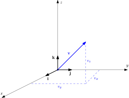Representation of a vector in $\mathbb{R}^3$

If $\mathsf{i},\mathsf{j}, \mathsf{k}$ represent the unit vectors along the $x,y,z$ axes, respectively, a vector $\mathsf{v}$ can be expressed uniquely as $\mathsf{v} = v_x \mathsf{i} + v_y \mathsf{j} + v_z \mathsf{k}$, where $v_x, v_y, v_z$ are the Cartesian components of the vector $\mathsf{v}$ (with respect to the basis vectors $\mathsf{i},\mathsf{j}$ and $\mathsf{k}$).

There are two core operations associated with vectors:

• Vector addition: Given two vectors $\mathsf{u} = u_x \mathsf{i} + u_y \mathsf{j} + u_z \mathsf{k}$ and $\mathsf{v} = v_x \mathsf{i} + v_y \mathsf{j} + v_z \mathsf{k}$, we can add them to get a new vector $\mathsf{u} + \mathsf{v}$, defined as $$\mathsf{u} + \mathsf{v} = (u_x + v_x) \mathsf{i} + (u_y + v_y) \mathsf{j} + (u_z + v_z) \mathsf{k}.$$ Geometrically, the new vector $\mathsf{u} + \mathsf{v}$ is obtained by placing the tail of $\mathsf{v}$ at the head of $\mathsf{u}$. The sum of the two vectors is then the vector which shares it’s tail with $\mathsf{u}$ and head with $\mathsf{v}$, as shown below:

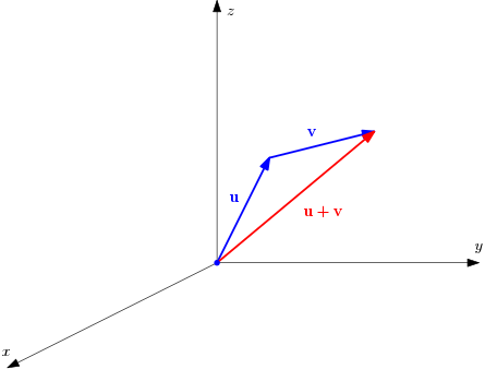  Vector addition in $\mathbb{R}^3$

  Note that we get the same vector independent of the order of addition: $\mathsf{u} + \mathsf{v} = \mathsf{v} + \mathsf{u}$. For this reason, vector addition is said to be commutative. It can also be shown easily that if $\mathsf{u}, \mathsf{v}, \mathsf{w}$ are three vectors, then $(\mathsf{u} + \mathsf{v}) + \mathsf{w} = \mathsf{u} + (\mathsf{v} + \mathsf{w})$. This property is called associativity.

• Scalar multiplication of a vector with a real number: Given any vector $\mathsf{v} = v_x \mathsf{i} + v_y \mathsf{j} + v_z \mathsf{k}$, we can multiply it by some real number $a$ to get the new vector that is $a$ times as long as $\mathsf{v}$: $a\mathsf{v}= av_x \mathsf{i} + av_y \mathsf{j} + av_z \mathsf{k}$. This is illustrated in the following figure:

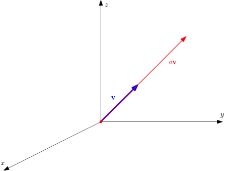  Scalar multiplication of a vector in $\mathbb{R}^3$

  Note that we will need only real vector spaces in what follows.

Some vector spaces admit an algebraic operation called the inner product. For instance, in three dimensional space, given two vectors $\mathsf{u} = u_x \mathsf{i} + u_y \mathsf{j} + u_z \mathsf{k}$ and $\mathsf{v} = v_x \mathsf{i} + v_y \mathsf{j} + v_z \mathsf{k}$, we can combine them using the dot product to produce a real number $\mathsf{u} \cdot \mathsf{v} = u_x v_x + u_y v_y + u_z v_z$. Using the dot product, it is customary to define the length or Euclidean norm of a vector $\mathsf{v} = v_x \mathsf{i} + v_y \mathsf{j} + v_z \mathsf{k}$ as the (non-negative) real number $\lVert \mathsf{v} \rVert = (\mathsf{v} \cdot \mathsf{v})^{\frac{1}{2}} = (v_x^2 + v_y^2 + v_z^2)^{\frac{1}{2}}$.

For vectors in three dimensional space (only), we also an additional important algebraic operation called the cross product: we can combine two vectors $\mathsf{u} = u_x \mathsf{i} + u_y \mathsf{j} + u_z \mathsf{k}$ and $\mathsf{v} = v_x \mathsf{i} + v_y \mathsf{j} + v_z \mathsf{k}$ using the cross product to obtain a new vector $\mathsf{u} \times \mathsf{v} = (u_y v_z - u_z v_y) \mathsf{i} + (u_z v_x - u_x v_z) \mathsf{j} + (u_x v_y - u_y v_x) \mathsf{k}$.

In what follows, we will first focus on just vector addition and scalar multiplication. These two operations embody a concept known as linearity, which is fundamental to appreciate what a vector is. We will then study inner product spaces, which are vector spaces with an additional structure known as an inner product, and highlight Euclidean spaces as an important example of inner product spaces.

Remark

The generalization of the cross product is known as the wedge product. We will not study the wedge product in detail in these notes since it is beyond the scope of these notes.

Notice that all the information about the vector $\mathsf{v} = v_x \mathsf{i} + v_y \mathsf{j} + v_z \mathsf{k}$ is contained in the ordered set of three real numbers $(v_x, v_y, v_z)$. What this means is that given any vector $\mathsf{v}$ in three dimensional space, we can uniquely associate with it a triple of real numbers, and vice versa. The set of all such ordered triples is the set $\mathbb{R}^3$, which is the set of all triples of real numbers. If we define addition of two such ordered triples and multiplication of an ordered triple with a real number as, $$\begin{gathered} (u_x, u_y, u_z) + (v_x, v_y, v_z) = (u_x + v_x, u_y + v_y, u_z + v_z), \nonumber\\ c(u_x, u_y, u_z) = (cu_x, cu_y, cu_z), \nonumber\end{gathered}$$ then the elements of $\mathbb{R}^3$, which are ordered triples of real numbers, behave exactly as the geometric picture of vectors as arrows that we just discussed, as far as the core properties of vector addition and scalar multiplication are concerned.

We now have two ways of representing a vector: as an arrow in three dimensional space, and as a set of ordered triple of real numbers. Both of these represent the same object. But the representation in terms of ordered tuples of real numbers immediately admits a generalization to cases where the pictorial representation fails. It is evident from the above discussion that there is nothing special about the number $3$ when we considered an ordered triple of real numbers. We can easily generalize this to a set of ordered $n$-tuple of real numbers $(u_1,u_2,\ldots,u_n) \in \mathbb{R}^n$, where $n \in \mathbb{N}$ could be any arbitrary positive integer. We can define addition and scalar multiplication in $\mathbb{R}^n$ analogous to the case of the ordered triples,

$$\begin{gathered} (u_1, u_2, \ldots, u_n) + (v_1, v_2, \ldots, v_n) = (u_1 + v_1, u_2 + v_2, \ldots, u_n + v_n), \label{eq:linearity_Rn_add}\\ a(u_1, u_2, \ldots, u_n) = (au_1, au_2, \ldots, au_n),\label{eq:linearity_Rn_sm}\end{gathered}$$

where $(u_1,u_2,\ldots,u_n)$ and $(v_1,v_2,\ldots,v_n)$ are two elements of $\mathbb{R}^n$, and $a$ is a real number. We will call this the standard linear structure on $\mathbb{R}^n$, and elements of $\mathbb{R}^n$ as vectors in $\mathbb{R}^n$. Note that there is no obvious way to picture an arrow in the $n$-dimensional space $\mathbb{R}^n$ for $n > 3$. Thus, by choosing the right representation, we can extend the elementary notion of vectors as quantities with magnitude and direction to more general objects.

Linear structure

Let us now generalize the previous discussion to define abstract vector spaces. Suppose that $V$ is a set such that it is possible to define two maps $$\begin{split} +:V \times V \to V; & \quad +(\mathsf{u},\mathsf{v}) \mapsto \mathsf{u} + \mathsf{v},\\ \cdot:V \times V \to V; & \quad \cdot(a, \mathsf{u}) \mapsto a\mathsf{u}, \end{split}$$ called vector addition and scalar multiplication, respectively, in $V$, that satisfy the following properties: for any $\mathsf{u}, \mathsf{v}, \mathsf{w} \in V$ and $a,b \in \mathbb{R}$,

1. Associativity of addition: $\mathsf{u} + (\mathsf{v} + \mathsf{w}) = (\mathsf{u} + \mathsf{v}) + \mathsf{w}$,

2. Commutativity of addition: $\mathsf{u} + \mathsf{v} = \mathsf{v} + \mathsf{u}$,

3. Existence of additive identity: there exists a unique element $\mathsf{0} \in V$, called the additive identity of $V$ such that $\mathsf{u} + \mathsf{0} = \mathsf{u}$,

4. Existence of additive inverse: for every $\mathsf{u} \in V$, there exists a unique element $-\mathsf{u} \in V$ such that $\mathsf{u} + (-\mathsf{u}) = \mathsf{0}$,

5. Distributivity of scalar multiplication over vector addition: $a(\mathsf{u} + \mathsf{v}) = a\mathsf{u} + a\mathsf{v}$,

6. Distributivity of scalar multiplication over scalar addition: $(a + b)\mathsf{u} = a\mathsf{u} + b\mathsf{u}$,

7. Compatibility of scalar multiplication with field multiplication: $a(b\mathsf{u}) = (ab)\mathsf{u}$,

8. Scaling property of scalar multiplication: $1\mathsf{u} = \mathsf{u}$.

A set $V$ that has two maps that satisfy these axioms is called a (real) vector space, or a (real) linear space. What we have accomplished through these axioms is to endow a set with a notion of addition that allows us to add two elements of the set to get a third element. We have also provided a mechanism to multiply a member of this set by a real number to get another element of this set. The maps $+$ and $\cdot$ are said to provide a linear structure on $V$. Elements of $V$ are called vectors.

Remark

Some textbooks mention additional closure axioms that indicate that if $\mathsf{u}, \mathsf{v} \in V$, then $\mathsf{u} + \mathsf{v} \in V$, and given any $\mathsf{u} \in V$ and $a \in \mathbb{R}$, $a \mathsf{u} \in V$. We don’t specify this explicitly since this is already implied by the function definitions $+:V \times V \to V$ and $\cdot:\mathbb{R} \times V \to V$. As mentioned in the previous discussion on set theory, we will always insist on mentioning the domain and codomain of every map/function we encounter. Hence, the so-called closure axioms are redundant for our purposes.

Remark

Following standard convention, we will often use the shorthand notation $\mathsf{u} - \mathsf{v}$ for $\mathsf{u} + (-\mathsf{v})$.

Example

The simplest example of a real vector space is the set of real numbers $\mathbb{R}$ with addition and multiplication defined in the standard manner. More generally, consider the set $\mathbb{R}^n$ consisting of all $n$-tuples of real numbers: $$\mathbb{R}^n = \{(u_1, \ldots, u_n)\,|\,\forall\,i=1,\ldots,n, \; u_i \in \mathbb{R}\}.$$ Given $(u_1, \ldots, u_n) \in \mathbb{R}^n$, $(v_1, \ldots, v_n) \in \mathbb{R}^n$, and $a \in \mathbb{R}$, let us define addition $+:\mathbb{R}^n \times \mathbb{R}^n \to \mathbb{R}^n$ and scalar multiplication $\cdot:\mathbb{R}\times \mathbb{R}^n \to \mathbb{R}^n$ as $$\begin{split} (u_1, \ldots, u_n) + (v_1, \ldots, v_n) &= (u_1 + v_1, \ldots, u_n + v_n),\\ a \cdot (u_1, \ldots, u_n) &= (au_1, \ldots, au_n). \end{split}$$ It is straightforward to verify that with addition and scalar multiplication thus defined, the triple $(\mathbb{R}^n,+,\cdot)$ is a real vector space. Note that the additive identity in $\mathbb{R}^n$ is the zero vector $(0, \ldots, 0) \in \mathbb{R}^n$, and the additive inverse of $(u_1, \ldots, u_n) \in \mathbb{R}^n$ is $(-u_1, \ldots, -u_n) \in \mathbb{R}^n$.

Example

Consider the set $\mathbb{R}^{m \times n}$ of all $m \times n$ matrices with real entries and defined addition of matrices and scalar mutliplication of a matrix with a real number in the usual sense (see Appendix ). It is easily checked that the set of all $m \times n$ matrices is a vector space. The zero vector in $\mathbb{R}^{m\times n}$ is the matrix with zero in all of its entries, and the additive inverse of a given matrix is just its negative.

Example

The definition of vector spaces admits more general kinds of objects. As a simple example, consider the set $C^0(\mathbb{R},\mathbb{R})$ consisting of all real-valued and continuous functions of one real variable. Given any $f, g \in C^0(\mathbb{R},\mathbb{R})$, and any $a \in \mathbb{R}$, we can define addition and scalar multiplication pointwise as follows: for any $x \in \mathbb{R}$, $$\begin{split} (f + g)(x) &= f(x) + g(x),\\ (a\cdot f)(x) &= a \, f(x). \end{split}$$ It is not difficult to verify that $(C^0(\mathbb{R},\mathbb{R}), +, \cdot)$ is a real vector space. The additive identity in $C^0(\mathbb{R},\mathbb{R})$ is the zero function $0 \in C^0(\mathbb{R},\mathbb{R})$ defined as follows: for any $x \in \mathbb{R}$, $0(x) = 0$. The additive inverse of $f \in C^0(\mathbb{R},\mathbb{R})$ is the function $-f \in C^0(\mathbb{R},\mathbb{R})$ defined as follows: for any $x \in \mathbb{R}$, $(-f)(x) = -f(x)$.

Subspaces and linear independence

A subset $U \subseteq V$ of a vector space $V$ is said to be a linear subspace of $V$ if $U$ is also a vector space. Note that it is implicitly assumed that both $U$ and $V$ share the operations of vector addition and scalar multiplication. It can be easily checked that if a subset $U \subseteq V$ of a real vector space $V$ has the property that for any $\mathsf{u}, \mathsf{v} \in U$, and any $a,b \in \mathbb{R}$, $(a\mathsf{u} + b\mathsf{v}) \in U$, then $U$ is a linear subspace of $V$. This property is often used to check if a given subset of a vector space is a linear subspace. An immediate consequence of this is the fact that every linear subspace of a given vector space must contain the additive identity $\mathsf{0} \in V$.

Example

Consider the following subsets of $\mathbb{R}^3$: $$\begin{split} S_1 &= \{(x,y,z) \in \mathbb{R}^3 \,|\, x + y + z = 0\},\\ S_2 &= \{(x,y,z) \in \mathbb{R}^3 \,|\, x + y + z = 1\},\\ S_3 &= \{(x,y,z) \in \mathbb{R}^3 \,|\, y = z = 0\}. \end{split}$$ To see that $S_1$ is a linear subspace of $\mathbb{R}^3$, note that if $(x_1, y_1, z_1) \in S_1$, $(x_2, y_2, z_2) \in S_1$, and $a, b \in \mathbb{R}$, then $a(x_1, y_1, z_1) + b(x_2, y_2, z_2) = ((ax_1 + bx_2), (ay_1 + by_2), (az_1 + bz_2)) \in \mathbb{R}^3$. Since $(ax_1 + bx_2) + (ay_1 + by_2) + (az_1 + bz_2) = a(x_1 + y_1 + z_1) + b(x_2 + y_2 + z_2) = (0,0,0)$, we see that $((ax_1 + bx_2), (ay_1 + by_2), (az_1 + bz_2)) \in S_1$. This shows that $S_1$ is indeed a linear subspace of $\mathbb{R}^3$. It is likewise verified that $S_3$ is also a linear subspace $\mathbb{R}^3$, while $S_2$ is not.

The intersection of two linear subspaces is also a linear subspace. Moreover, any finite intersection of linear subspaces of a vector space $V$ is also a linear subspace of $V$, as can be easily checked.

Example

In the previous example, the intersection of the subspaces $S_1 = \{(x,y,z) \in \mathbb{R}^3 \,|\, x + y + z = 0\}$ and $S_3 = \{(x,y,z) \in \mathbb{R}^3 \,|\, y = z = 0\}$ of $\mathbb{R}^3$ is easily seen to be $$S_1 \cap S_3 = \{(0,0,0)\},$$ which is the trivial subspace of $\mathbb{R}^3$.

Two non-zero vectors $\mathsf{u},\mathsf{v} \in V$ in a vector space $V$ are said to be linearly independent iff $a\mathsf{u} + b\mathsf{v} = 0$, where $a,b$ are real numbers, implies that $a=0$ and $b=0$. Thus $\mathsf{u}$ and $\mathsf{v}$ are linearly independent iff the only linear combination of $\mathsf{u}$ and $\mathsf{v}$ that yields $\mathsf{0}$ is the trivial linear combination $0\mathsf{u} + 0\mathsf{v}$. If this is not true, then $\mathsf{u}$ and $\mathsf{v}$ are said to be linearly dependent. This definition can be easily extended to a finite set of non-zero vectors $\mathsf{v}_1, \mathsf{v}_2, \ldots, \mathsf{v}_n$, where $n \in \mathbb{N}$. Thus, the set of vectors $\mathsf{v}_1, \mathsf{v}_2, \ldots, \mathsf{v}_n$ in $V$ is said to be linearly independent iff the only real numbers $a_1, a_2, \ldots, a_n$ that satisfy the equation $$\sum_{i=1}^n a_i \mathsf{v}_i = 0,$$ are $a_1 = a_2 = \ldots = a_n = 0$.

Example

Consider the vectors $\mathsf{v}_1 = (1,2) \in \mathbb{R}^2$ and $\mathsf{v}_2 = (2,3)\in\mathbb{R}^2$ in the two dimensional Euclidean space $\mathbb{R}^2$. For real numbers $a, b \in \mathbb{R}$, note that $$a\mathsf{v}_1 + b\mathsf{v}_2 = 0 \quad\Rightarrow\quad (a + 2b, 2a + 3b) = (0,0).$$ Solving the equations $a + 2b = 0$ and $2a + 3b = 0$, we immediately see that $a = b = 0$, which shows that $\mathsf{v}_1$ and $\mathsf{v}_2$ are linearly independent vectors in $\mathbb{R}^2$. If $\mathsf{v}_3 = (2,4) \in \mathbb{R}^2$, then $\mathsf{v}_1$ and $\mathsf{v}_3$ are linearly dependent since if for $a, b \in \mathbb{R}$, $$a\mathsf{v}_1 + b\mathsf{v}_3 = 0 \quad\Rightarrow\quad (a + 2b, 2a + 4b) = (0,0).$$ These equations do not imply that $a = b = 0$. For instance, $a = -2, b = 1$ satisfies the condition. We thus see that $\mathsf{v}_1$ and $\mathsf{v}_3$ are linearly dependent.

Basis of a vector space

We will now introduce a very important tool called the basis of a vector space. The basic idea is that once we identify a basis for a vector space, we can use the linear structure inherent in the space to reduce all computations related to the vector space as a whole, to just computations on the basis set. We will need a few definitions first in order to define the basis.

The linear span of a set of vectors $\{\mathsf{v}_1, \mathsf{v}_2, \ldots, \mathsf{v}_m\}$ in $V$, written as $\text{span}(\{\mathsf{v}_1,\ldots,\mathsf{v}_m\})$, is defined as the set of all it’s linear combinations: $$\text{span}(\{\mathsf{v}_1,\ldots,\mathsf{v}_m\}) = \left\{\sum_{i=1}^m a_i \mathsf{v}_i \,\bigg\vert\, \forall\,1\le i\le m,\,a_i \in \mathbb{R}\right\}.$$ It is also common to refer to the linear span as just the span. It is straightforward to check that the linear span of any finite collection of vectors in a vector space $V$ is a linear subspace of the vector space $V$.

Example

Let us consider the vectors $\mathsf{v}_1 = (1,2,3) \in \mathbb{R}^3$ and $\mathsf{v}_2 = (2,3,4) \in \mathbb{R}^3$ in $\mathbb{R}^3$. The span of these two vectors is the following subset of $\mathbb{R}^3$: $$\text{span}(\{\mathsf{v}_1, \mathsf{v}_2\}) = \{((a + 2b, 2a + 3b, 3a + 4b) \in \mathbb{R}^3 \,|\, a, b \in \mathbb{R}\}.$$ It is left as an easy exercise to verify that this is indeed a linear subspace of $\mathbb{R}^3$.

An ordered subset $S \subseteq V$ a vector space $V$ is said to constitute a basis of $V$ if

1. $S$ is linearly independent, and

2. $\text{span}(S) = V$.

In the special case when a vector space $V$ is spanned by a finite ordered set of vectors $(\mathsf{v}_1, \ldots, \mathsf{v}_n) \subseteq V$, for some $n \in \mathbb{N}$, the vector space $V$ is said to be finite dimensional, and the number $n$ is called the dimension of the vector space $V$ (written $\text{dim}(V)$). A vector space that is not finite dimensional is said to be infinite dimensional. In what follows, we will only deal with finite dimensional vector spaces.

If $V$ is an $n$-dimensional vector space, and $(\mathsf{v}_1, \ldots, \mathsf{v}_n)$ is a basis for $V$, then we will often abbreviate the basis as $(\mathsf{v}_i)_{i=1}^n$, or just $(\mathsf{v}_i)$, when the dimension $n$ is evident from the context.

Example

Let us revisit the $n$-dimensional Euclidean space $\mathbb{R}^n$, and consider the following vectors: for any $1 \le i \le n$, $$\mathsf{e}_i = (0, \ldots, \underbrace{1}_{i^{\text{th}}\text{ position}}, \ldots 0).$$ It is easy to check that the $(\mathsf{e}_1, \ldots, \mathsf{e}_n)$ is a basis of $\mathbb{R}^n$. In particular, note that any $(u_1, \ldots, u_n) \in \mathbb{R}^n$ can be written as $$(u_1, \ldots, u_n) = u_1(1, 0, \ldots, 0) + \ldots + u_n(0, \ldots, 0, 1) = \sum_{i=1}^n u_i \mathsf{e}_i.$$ The ordered set $(\mathsf{e}_i)_{i=1}^n$ is called the standard basis of $\mathbb{R}^n$. Note that in the special case of $\mathbb{R}^3$, the set of basis vectors $(\mathsf{e}_1,\mathsf{e}_2,\mathsf{e}_3)$ is identical to the basis set $(\mathsf{i},\mathsf{j},\mathsf{k})$ introduced in the beginning of this section.

Given a vector space $V$ of dimension $n$, it is possible to choose an infinite number of bases for $V$. This non-uniqueness in the choice of the basis can be easily understood as follows. Pick any $\mathsf{g}_1 \in V$. Choose $\mathsf{g}_2$ from the set $V \setminus \text{span}({\mathsf{g}_1})$, $\mathsf{g}_3$ from the set $V \setminus \text{span}({\mathsf{g}_1, \mathsf{g}_2})$, and so on. This process will terminate in $n$ steps since the vector space $V$ is of dimension $n$. The resulting set of vectors $(\mathsf{g}_1, \ldots, \mathsf{g}_n)$ is a basis for $V$.

Inner products and norms

We will now introduce a special additional structure on an abstract vector space $V$ called the inner product. There are two reasons for introducing the inner product right at the outset: first, the mathematical development becomes significantly simpler, and second, many important applications in science and engineering can be studied in this setting.

Remark

There is an elegant theory of abstract linear spaces, both in the finite and infinite dimensional cases, where inner products are not defined. We will however not develop this general theory here.

Given a vector space $V$, an inner product on $V$ is defined as a map of the form $g:V \times V \to \mathbb{R}$ such that, for any $\mathsf{u}, \mathsf{v}, \mathsf{w} \in V$ and $a,b \in \mathbb{R}$,

1. Symmetry: $g(\mathsf{u},\mathsf{v}) = g(\mathsf{v},\mathsf{u})$,

2. Bilinearity: $g(\mathsf{u},(a \mathsf{v} + b \mathsf{w})) = a g(\mathsf{u},\mathsf{v}) + b g(\mathsf{u},\mathsf{w})$,

3. Positive definiteness: $g(\mathsf{u},\mathsf{u}) \ge 0$, and $g(\mathsf{u},\mathsf{u}) = 0$ iff $\mathsf{u} = \mathsf{0}$.

A vector space $V$ endowed with a map $\cdot:V \times V \to \mathbb{R}$ that satisfies the three properties mentioned above is said to be an inner product space. All vector spaces considered henceforth will be assumed to be inner product spaces, unless stated otherwise.

Remark

Given $\mathsf{u}, \mathsf{v} \in V$, we will often write $g(\mathsf{u}, \mathsf{v})$ as just $\mathsf{u} \cdot \mathsf{v}$, with the understanding that the inner product $g$ is evident from the context.

Example

The simplest, and also the most important, example of an inner product space is the vector space $\mathbb{R}^n$ defined earlier, with the inner product $\cdot:V \times V \to \mathbb{R}$ defined as follows: for any $(u_1, \ldots, u_n) \in \mathbb{R}^n$ and $(v_1, \ldots, v_n) \in \mathbb{R}^n$, $$(u_1, \ldots, u_n) \cdot (v_1, \ldots, v_n) = \sum_{i=1}^n u_i v_i.$$ It is easy to check that this is indeed an inner product. The vector space $\mathbb{R}^n$ with this inner product is called the Euclidean space of dimension $n$. We will use the same symbol $\mathbb{R}^n$ to denote the $n$-dimensional Euclidean space.

Example

Define the set $\mathcal{P}_n([a,b],\mathbb{R})$ as the set of all real valued polynomials of degree less than or equal to $n$ on the interval $[a,b] \subseteq \mathbb{R}$: $$\mathcal{P}_n([a,b],\mathbb{R}) = \{f:[a,b] \subseteq\mathbb{R} \to \mathbb{R} \,|\, \forall\,x \in [a,b], \; f(x) = a_0 + a_1 x + \ldots + a_n x^n, \text{ where } a_0, a_1, \ldots, a_n \in \mathbb{R}\}.$$ Define the function $\cdot:\mathcal{P}_n([a,b],\mathbb{R}) \times \mathcal{P}_n([a,b],\mathbb{R}) \to \mathbb{R}$ as follows: for any $f,g \in \mathcal{P}_n([a,b],\mathbb{R})$, $$f \cdot g = \int_a^b f(x)g(x) \, dx.$$ It is left as a simple exercise to verify that this function is actually an inner product on the linear space $\mathcal{P}_n([a,b],\mathbb{R})$ with addition and scalar multiplication defined pointwise.

The inner product on a vector space $V$ can be used to define a norm on $V$. A norm on a vector space $V$ is a function of the form $\lVert \cdot \rVert:V \to \mathbb{R}$ such that, for any $\mathsf{u}, \mathsf{v} \in V$ and $a \in \mathbb{R}$,

1. Positive definiteness: $\lVert \mathsf{u} \rVert \ge 0$, and $\lVert \mathsf{u} \rVert = 0$ iff $\mathsf{u} = \mathsf{0}$,

2. Homogeneity: $\lVert a \mathsf{u} \rVert = |a| \lVert \mathsf{u} \rVert$,

3. Sub-additivity: $\lVert \mathsf{u} + \mathsf{v} \rVert \le \lVert \mathsf{u} \rVert + \lVert \mathsf{v} \rVert$.

Here, $|a|$ refers to the absolute value of $a \in \mathbb{R}$. The property of sub-additivity is also referred to as the triangle inequality.

A vector space $V$ equipped with a norm $\lVert \cdot \rVert:V \to \mathbb{R}$ that satisfies these properties is called a normed vector space, or a normed linear space. Note that every inner product space is a normed linear space. To see this, note that given an an inner product $\cdot:V \times V \to \mathbb{R}$, the norm $\lVert \cdot \rVert: V \to \mathbb{R}$ induced by this inner product is defined as follows: for any $\mathsf{v} \in V$, $$\lVert \mathsf{v} \rVert = \sqrt{\mathsf{v} \cdot \mathsf{v}}.$$ The norm induced by the Euclidean inner product on $\mathbb{R}^3$ is called the standard Euclidean norm on $\mathbb{R}^n$.

Remark

In general, a normed vector space is not an inner product space. If, however, the norm $\lVert \cdot \rVert:V \to \mathbb{R}$ on a normed vector space $V$ satisfies the following relation, called the parallelogram identity, $$\frac{1}{2}\left(\lVert \mathsf{u} + \mathsf{v} \rVert^2 + \lVert \mathsf{u} - \mathsf{v}\rVert^2\right) = \lVert \mathsf{u} \rVert^2 + \lVert \mathsf{v} \rVert^2,$$ for any $\mathsf{u}, \mathsf{v} \in V$, then it is possible to define an inner product $\cdot:V \times V \to \mathbb{R}$ using the norm as follows: for any $\mathsf{u},\mathsf{v} \in V$, $$\mathsf{u} \cdot \mathsf{v} = \frac{1}{4}\left(\lVert \mathsf{u} + \mathsf{v} \rVert^2 - \lVert \mathsf{u} - \mathsf{v}\rVert^2\right).$$ This relation is called the polarization identity.

Example

Let us consider the $n$-dimensional Euclidean space $\mathbb{R}^n$ with the standard inner product, defined earlier. The norm of a vector $(x_1, \ldots, x_n) \in \mathbb{R}^n$ is easily computed as $$\lVert (x_1, \ldots, x_n) \rVert^2 = \sum_{i=1}^n x_i^2.$$ This norm is called the standard Euclidean norm, or the $L_2$-norm on $\mathbb{R}^n$.

A variety of other norms can be defined on a given inner product space. For instance, the $L_p$-norm on $\mathbb{R}^n$ can be defined as follows: for any $(x_1, \ldots, x_n) \in \mathbb{R}^n$ and $1 \le p < \infty$, $$\lVert (x_1, \ldots, x_n) \rVert_p = \left(\sum_{i=1}^n x_i^p\right)^{\frac{1}{p}}.$$ The $L_\infty$-norm on $\mathbb{R}^n$ is defined as $$\lVert (x_1, \ldots, x_n) \rVert_\infty = \text{max } \{x_1, \ldots, x_n\}.$$ Note that the standard Euclidean norm corresponds to $\lVert \cdot \lVert_2$.

Remark

There is an important theorem that states that all norms on a finite dimensional vector space are equivalent. This means the following: given norms $\lVert \cdot \rVert_1:V \to \mathbb{R}$ and $\lVert \cdot \rVert_2:V \to \mathbb{R}$ on a finite dimensional vector space $V$, there exists constants $c_L, c_U \in \mathbb{R}$ such that, for any $\mathsf{v} \in V$, $$c_L \lVert \mathsf{v} \rVert_2 \le \lVert \mathsf{v} \rVert_1 \le c_U \lVert \mathsf{v} \rVert_2.$$ Without getting into technical details, this roughly means that the conclusions we draw about topological notions in a normed vector space are independent of the specific norm chosen.

Cauchy-Schwarz inequality

Let $V$ be a real vector space equipped with an inner product $\cdot:V \times V \to \mathbb{R}$. An important property of inner products that turns out to be quite useful in practice is discussed now. Given any $\mathsf{u}, \mathsf{v} \in V$, the Cauchy-Schwarz inequality states that $$|\mathsf{u} \cdot \mathsf{v}| \le \lVert \mathsf{u} \rVert \lVert \mathsf{v} \rVert.$$ Furthermore, the equality holds iff $\mathsf{u}$ and $\mathsf{v}$ are linearly dependent. The proof of the Cauchy-Schwarz inequality is quite easy: for any $\mathsf{u}, \mathsf{v} \in V$, and $a \in \mathbb{R}$, $$\lVert \mathsf{u} + a \mathsf{v} \rVert^2 \ge 0 \Rightarrow \lVert \mathsf{u} \rVert^2 + 2a \mathsf{u} \cdot \mathsf{v} + a^2\rVert \mathsf{v} \rVert^2 \ge 0.$$ Substituting $$a = -\frac{\mathsf{u} \cdot \mathsf{v}}{\lVert \mathsf{v} \rVert^2}$$ in this inequality, we get $$(\mathsf{u} \cdot \mathsf{v})^2 \le \lVert \mathsf{u} \rVert^2 \lVert \mathsf{v} \rVert^2,$$ which immediately yields the Cauchy-Schwartz inequality. To prove the second part, note that if $\mathsf{u}$ and $\mathsf{v}$ are linearly dependent, then, without loss of generality, $\mathsf{v} = a\mathsf{u}$ for some $a \ in \mathbb{R}$. In this case, $\mathsf{u} \cdot \mathsf{v} = \lvert a \rvert \lVert \mathsf{u} \rVert^2 = \lVert \mathsf{u} \rVert \lVert \mathsf{v} \rVert$. On the other hand, if $\mathsf{u} \cdot \mathsf{v} = \lVert \mathsf{u} \rVert \lVert \mathsf{v} \rVert$, consider the vector $\mathsf{w} \in V$, where, $$\mathsf{w} = \mathsf{u} - \frac{\lVert \mathsf{u} \rVert}{\lVert \mathsf{v} \rVert}\mathsf{v}.$$ It is straightforward to show that $\lVert \mathsf{w} \rVert = 0$, and hence that $\mathsf{w} = 0$. This shows that $\mathsf{u}$ and $\mathsf{v}$ are linearly dependent. The Cauchy-Schwartz inequality is thus proved.

The angle $\theta:V \times V \to \in [0,2\pi) \subseteq \mathbb{R}$ between two vectors $\mathsf{u}, \mathsf{v} \in V$ is defined via the relation $$\cos \theta(\mathsf{u},\mathsf{v}) = \frac{\mathsf{u} \cdot \mathsf{v}}{\lVert \mathsf{u} \rVert\lVert \mathsf{v} \rVert}.$$ Note how the Cauchy-Schwarz inequality implies that this definition is well-defined. If the angle between two vectors $\mathsf{u}, \mathsf{v} \in V$ is $\pi/2$, they are said to be orthogonal. Equivalently, $\mathsf{u}, \mathsf{v} \in V$ are said to be orthogonal if $\mathsf{u} \cdot \mathsf{v} = 0$. If $\mathsf{u}, \mathsf{v} \in V$ are orthogonal, and if it is further true that $\lVert \mathsf{u} \rVert = \lVert \mathsf{v} \rVert = 1$, then $\mathsf{u}$ and $\mathsf{v}$ are said to be orthonormal.

Example

The vectors $\mathsf{u} = (1, \sqrt{3}) \in \mathbb{R}^2$ and $\mathsf{v} = (-\sqrt{3}, 1) \in \mathbb{R}^2$ are orthogonal since $\mathsf{u} \cdot \mathsf{v} = 0$. They are not orthonormal since $\lVert \mathsf{u} \rVert = \lVert \mathsf{v} \rVert = 2$. The vectors $\tilde{\mathsf{u}} = \mathsf{u}/\lVert \mathsf{u} \rVert = (1/2, \sqrt{3}/2) \in \mathbb{R}^2$ and $\mathsf{v} = \mathsf{v}/\lVert \mathsf{v} \rVert = (-\sqrt{3}/2, 1/2) \in \mathbb{R}^2$ are, however, orthonormal.

The following inequality also holds for any $\mathsf{u},\mathsf{v} \in V$ in an inner product space $V$: $$\lVert \mathsf{u} + \mathsf{v} \rVert \le \lVert \mathsf{u} \rVert + \lVert \mathsf{v} \rVert.$$ Recall that this is the triangle inequality. The triangle inequality is readily proved using the Cauchy-Schwarz inequality: for any $\mathsf{u}, \mathsf{v} \in V$: $$\begin{split} \lVert \mathsf{u} + \mathsf{v} \rVert^2 &= \lVert \mathsf{u} \rVert^2 + \lVert \mathsf{v} \rVert^2 + 2 \mathsf{u} \cdot \mathsf{v}\\ &\le \lVert \mathsf{u} \rVert^2 + \lVert \mathsf{v} \rVert^2 + 2 \lVert \mathsf{u} \rVert \lVert \mathsf{v} \rVert\\ &= (\lVert \mathsf{u} \rVert + \lVert \mathsf{v} \rVert)^2. \end{split}$$ The triangle inequality follows by taking the square root on both sides.

Gram-Schmidt orthogonalization

Let us now reconsider the notion of a basis of an $n$-dimensional vector space $V$ in the special case when the vector space also has an inner product $\cdot:V \times V \to \mathbb{R}$ defined on it. We say that a basis $(\mathsf{g}_i)$ of $V$ is orthogonal if $\mathsf{g}_i \cdot \mathsf{g}_j = 0$ whenever $i, j \in \{1, \ldots, n\}$, and $i \neq j$. If it is further true that $\mathsf{g}_i \cdot \mathsf{g}_i = 1$ for every $i \in \{1, \ldots, n\}$, we say that the basis $(\mathsf{g}_i)$ is orthonormal. The fact that a basis $(\mathsf{g}_i)$ of $V$ is orthonormal can be succinctly expressed by the following equation: for any $i,j \in \{1,\ldots,n\}$, $$\mathsf{g}_i \cdot \mathsf{g}_j = \delta_{ij},$$ where $\delta_{ij}$ is the Krönecker delta symbol that is defined as follows: $$\delta_{ij} = \begin{cases} 1, & i = j,\\ 0, & i \neq j. \end{cases}$$

Example

It is straightforward to verify that the standard basis $(\mathsf{e}_i)$ of $\mathbb{R}^n$ is an orthonormal basis, since it follows from the definition of the standard basis that $\mathsf{e}_i \cdot \mathsf{e}_j = \delta_{ij}$.

The Gram-Schmidt orthogonalization procedure is an algorithm that helps us to transform any given basis $(\tilde{\mathsf{g}}_i)$ of $V$ into an orthonormal basis $(\mathsf{g}_i)$. The algorithm works as follows:

• Let $$\mathsf{g}_1 = \frac{\tilde{\mathsf{g}}_1}{\lVert \tilde{\mathsf{g}}_1 \rVert}.$$

• We now define $\mathsf{g}_2$ by removing the component of $\tilde{\mathsf{g}}_2$ along the direction $\mathsf{g}_1$: $$\mathsf{g}_2 = \frac{\tilde{\mathsf{g}}_2 - (\tilde{\mathsf{g}}_2 \cdot \mathsf{g}_1)e_1}{\lVert \tilde{\mathsf{g}}_2 - (\tilde{\mathsf{g}}_2 \cdot \mathsf{g}_1)\mathsf{g}_1 \rVert}.$$ It is easy to check that $\mathsf{g}_2 \cdot \mathsf{g}_1 = 0$ and $\lVert \mathsf{g}_2 \rVert = 1$.

• We then obtain $\mathsf{g}_3$ in a similar manner by removing the components of $\tilde{\mathsf{g}}_3$ along $\mathsf{g}_1$ and $\mathsf{g}_2$: $$\mathsf{g}_3 = \frac{\tilde{\mathsf{g}}_3 - (\tilde{\mathsf{g}}_3 \cdot \mathsf{g}_2)\mathsf{g}_2 - (\tilde{\mathsf{g}}_3 \cdot \mathsf{g}_1)e_1}{\lVert \tilde{\mathsf{g}}_3 - (\tilde{\mathsf{g}}_3 \cdot \mathsf{g}_2)\mathsf{g}_2 - (\tilde{\mathsf{g}}_3 \cdot \mathsf{g}_1)\mathsf{g}_1 \rVert}.$$ It is straightforward to verify that $\mathsf{g}_1 \cdot \mathsf{g}_3 = 0$, $\mathsf{g}_2 \cdot \mathsf{g}_3 = 0$ and $\lVert \mathsf{g}_3 \rVert = 1$.

• Continuing this process, we can construct an orthonormal basis $(\mathsf{g}_i)_{i=1}^n$.

Example

As a simple illustration of the Gram-Schmidt orthogonalization process, let us consider the vectors $\tilde{\mathsf{g}}_1 = (1,2) \in \mathbb{R}^2$ and $\tilde{\mathsf{g}}_2 = (2,3) \in \mathbb{R}^2$. We verified earlier that these vectors are linearly independent, and that they form a basis of $\mathbb{R}^2$. They are however not orthogonal since $\tilde{\mathsf{g}}_1 \cdot \tilde{\mathsf{g}}_2 = 8 \neq 0$. Let us orthonormalize this basis using the Gram-Schmidt process. To start with, let us normalize $\tilde{\mathsf{g}}_1$: $$\mathsf{g}_1 = \frac{\tilde{\mathsf{g}}_1}{\lVert \tilde{\mathsf{g}}_1 \rVert} = \left(\frac{1}{\sqrt{5}}, \frac{2}{\sqrt{5}}\right) \in \mathbb{R}^2.$$ We can now construct $\mathsf{g}_2 \in \mathbb{R}^2$ by projecting out the component of $\tilde{\mathsf{g}}_2$ along $\mathsf{g}_1$: $$\begin{split} \mathsf{g}_2 &= \frac{\tilde{\mathsf{g}}_2 - (\tilde{\mathsf{g}}_2 \cdot \mathsf{g}_1)\mathsf{g}_1}{\lVert \tilde{\mathsf{g}}_2 - (\tilde{\mathsf{g}}_2 \cdot \mathsf{g}_1)\mathsf{g}_1 \rVert}\\ &= \frac{(2,3) - \left((2,3)\cdot(1/\sqrt{5},2/\sqrt{5})\right)(1/\sqrt{5},2/\sqrt{5})}{\lVert (2,3) - \left((2,3)\cdot(1/\sqrt{5},2/\sqrt{5})\right)(1/\sqrt{5},2/\sqrt{5})\rVert}\\ &= \frac{(2/5, -1/5)}{\lVert (2/5, -1/5) \rVert}\\ &= \left(\frac{2}{\sqrt{5}}, -\frac{1}{\sqrt{5}}\right) \in \mathbb{R}^2. \end{split}$$ It is easily checked that $\lVert \mathsf{g}_1 \rVert = 1$ and $\lVert \mathsf{g}_2 \rVert = 1$, and that $$\mathsf{g}_1 \cdot \mathsf{g}_2 = \left(\frac{1}{\sqrt{5}}, \frac{2}{\sqrt{5}}\right) \cdot \left(\frac{2}{\sqrt{5}}, -\frac{1}{\sqrt{5}}\right) = 0.$$ We have thus constructed an orthonormal basis $(\mathsf{g}_1, \mathsf{g}_2)$ of $\mathbb{R}^2$ starting from the general basis $(\tilde{\mathsf{g}}_1, \tilde{\mathsf{g}}_2)$ of $\mathbb{R}^2$ by following the Gram-Schmidt algorithm.

Note that the orientation of the basis $(\mathsf{g}_1, \mathsf{g}_2)$ obtained here is the opposite of the orientation of the standard basis $(\mathsf{e}_1, \mathsf{e}_2)$. To see this, embed these vectors in $\mathbb{R}^3$ to get the vectors $\mathsf{e}_1 = (1,0,0)$, $\mathsf{e}_2 = (0,1,0)$, $\mathsf{g}_1 = (1/\sqrt{5}, 2/\sqrt{5}, 0)$, $\mathsf{g}_2 = (2/\sqrt{5}, -1/\sqrt{5}, 0)$, and note that $\mathsf{e}_1 \times \mathsf{e}_2 = \mathsf{e}_3$, whereas $\mathsf{g}_1 \times \mathsf{g}_2 = -\sqrt{5} \hat{e}_3$ - they have opposite signs! This doesn’t really affect the Gram-Schmidt algorithm because if $(\mathsf{g}_1, \mathsf{g}_2)$ is a basis of $\mathbb{R}^2$, then so is $(\mathsf{g}_2, \mathsf{g}_1)$.

Remark

It turns out that the choice of an orthonormal basis is sufficient for most applications. In the discussion below, we will first study various concepts with respect to the choice of an orthonormal basis, since the calculations are much simpler in this case. The general case of arbitrary bases will be discussed after this to give an idea of how some calculations can be more involved with respect to general bases.

Basis representation of vectors

We will now study the representation of a vector $\mathsf{v} \in V$ in an $n$-dimensional inner product space $V$ with respect to an orthonormal basis $(\mathsf{e}_1, \ldots, \mathsf{e}_n)$ of $V$. It is worth reiterating that we will only deal with orthonormal bases unless otherwise stated.

The fact that $(\mathsf{e}_1, \ldots, \mathsf{e}_n)$ is a basis of $V$ implies that every $\mathsf{v} \in V$ can be written as $$\mathsf{v} = \sum_{i=1}^n v_i \mathsf{e}_i$$ where $v_i \in \mathbb{R}$ for every $i \in \{1, \ldots, n\}$. This is called the representation of $v$ with respect to the basis $(\mathsf{e}_1, \ldots, \mathsf{e}_n)$. The real numbers $v_1, \ldots v_n$ are called the components of $\mathsf{v}$ with respect to the basis $(\mathsf{e}_1, \ldots, \mathsf{e}_n)$.

To compute the components $v_i$, we can exploit the fact that $(\mathsf{e}_i)$ is an orthonormal basis: $$\mathsf{v} \cdot \mathsf{e}_j = v_j \quad\Rightarrow\quad \mathsf{v} = \sum (\mathsf{v} \cdot \mathsf{e}_i) \mathsf{e}_i.$$ The components $v_i$ thus computed are unique since we have explicitly constructed each component $v_i$ as $\mathsf{v} \cdot \mathsf{e}_i$. We can alternatively show the uniqueness of the components based on the fact that the basis vectors are linearly independent by definition.

Remark

Notice how we have represented the sum on the right without representing the summation index, and the range of summation. We will write $\sum_i$, or just $\sum$ in place of $\sum_{i=1}^n$, whenever the range under consideration is obvious from the context. If no index is associated with the summation symbol, as in $\sum$, it will be assumed that the sum is with respect to all repeating indices. In addition, we will assume that the range of the all the indices involved is known from the context. While on this, it is worth noting that many authors employ the Einstein summation convention, according to which, a sum of the form $\sum u_i \mathsf{e}_i$ is written simply as $u_i \mathsf{e}_i$, with the summation over $i$ being implicitly understood as long as the indices repeat twice. For pedagogical reasons, we will not follow the Einstein summation convention in these notes.

Example

As a trivial example of the basis representation of a vector, consider any $(x_1, \ldots, x_n) \in \mathbb{R}^n$. This vector can be written with respect to the standard basis $(\mathsf{e}_i)$ of $\mathbb{R}^n$ as $$(x_1, \ldots, x_n) = \sum x_i \mathsf{e}_i.$$ Notice that $x_i = (x_1, \ldots, x_n) \cdot \mathsf{e}_i$.

Example

As a non-trivial, yet simple, example of basis representation of a vector, consider the orthonormal basis $(\mathsf{g}_1, \mathsf{g}_2)$ of $\mathbb{R}^2$, where $\mathsf{g}_1 = (2/\sqrt{5}, -1/\sqrt{5})$ and $\mathsf{g}_2 = (1/\sqrt{5}, 2/\sqrt{5})$ - notice that we have swapped the order of the basis constructed earlier in the context of the Gram-Schmidt procedure to maintain orientation. Consider any $(x_1, x_2) \in \mathbb{R}^2$, we can express this in terms of the basis $(\mathsf{g}_1, \mathsf{g}_2)$ as $$(x_1, x_2) = \sum \bar{x}_i \mathsf{g}_i,$$ for some real constants $(\bar{x}_i)$. To compute this, note that we can write $(x_1, x_2) = \sum x_i \mathsf{e}_i$ using the standard basis of $\mathbb{R}^2$. The constants $(\bar{x}_i)$ are easily computed by taking the appropriate dot products: $$\begin{split} \bar{x}_i &= \left(\sum x_j \mathsf{e}_j\right)\cdot \mathsf{g}_i\\ &= (\mathsf{g}_i \cdot \mathsf{e}_1) x_1 + (\mathsf{g}_i \cdot \mathsf{e}_2) x_2. \end{split}$$ For instance, the vector $(1,2) \in \mathbb{R}^2$ can be expressed in terms of the $(\mathsf{g}_1, \mathsf{g}_2)$ basis as $(1,2) = \sum \bar{x}_i \mathsf{g}_i$, where $$\begin{split} \bar{x}_1 &= \frac{2}{\sqrt{5}}1 - \frac{1}{\sqrt{5}}2 = 0,\\ \bar{x}_2 &= \frac{1}{\sqrt{5}}1 + \frac{2}{\sqrt{5}}2 = \sqrt{5}. \end{split}$$ We thus see that $(1,2) = \sqrt{5}\mathsf{g}_2$, a fact that can be easily checked directly.

We will now introduce a useful notion called component maps to collect the components $v_i$ of any $\mathsf{v} \in V$ with respect to the (not necessarily orthonormal) basis $B = (\mathsf{e}_1, \ldots, \mathsf{e}_n)$ of $V$. Define the component map $\mathsf\phi_{V,B}:V \to \mathbb{R}^n$ as follows: $$\phi_{V,B}(\mathsf{v}) = [v_1, \ldots, v_n]^T.$$ Notice how we have collected together the components of $\mathsf{v}$ as a column vector of size $n$ using the component map. It is useful at this point to introduce the following notation: $$[\mathsf{v}]_{(\mathsf{e}_i)} = [v_1, \ldots, v_n]^T$$ When the choice of basis is evident from the context, we will often write $[\mathsf{v}]_{(\mathsf{e}_i)}$ as just $[\mathsf{v}]$. We can thus alternatively the basis representation of any $\mathsf{v} \in V$ with respect to a general basis $(\mathsf{e}_i)$ of $V$ as follows: $$\mathsf{v} = \sum v_i \mathsf{e}_i = \sum \left(\mathsf\phi_{V,B}(\mathsf{v})\right)_i \mathsf{e}_i = \sum [\mathsf{v}]_i \mathsf{e}_i.$$ We will however use the simpler notation $\mathsf{v} = \sum v_i \mathsf{e}_i$, and use the $[\mathsf{v}]$ notation only when we want to refer to the components alone as a column vector. We will see shortly that the component map is an example of an isomorphism between the vector spaces $V$ and $\mathbb{R}^n$.

Remark

We will often write the component map $\mathsf\phi_{V,B}$ as $\mathsf\phi_V$, or just $\mathsf\phi$, when the vector space and its basis are evident from the context. At times, we will omit $\mathsf\phi$ altogether and refer to the component map using the following notation: $\mathsf{v} \in V \mapsto [\mathsf{v}] \in \mathbb{R}^n$.

Example

As a quick illustration of this, notice that the vector $(1,2) \in \mathbb{R}^2$ has the following matrix representation with respect to the orthonormal basis $(e_1, e_2)$, where $e_1 = (2/\sqrt{5}, -1/\sqrt{5})$ and $e_2 = (1/\sqrt{5}, 2/\sqrt{5})$ of $\mathbb{R}^2$ is $[0,\sqrt{5}]^T$.

Change of basis rules for vectors

Given an $n$-dimensional inner product space $V$, let us first consider the case where $(\mathsf{e}_i)$ and $(\mathsf{g}_i)$ are two general bases of $V$, not necessarily orthonormal. Then, any $\mathsf{v} \in V$ can be written as $$\mathsf{v} = \sum v_i \mathsf{e}_i = \sum \tilde{v}_i \mathsf{g}_i,$$ where $(v_i)$ and $(\tilde{v}_i)$ are the components of $\mathsf{v}$ with respect to the bases $(\mathsf{e}_i)$ and $(\mathsf{g}_i)$, respectively. The fact that $(\mathsf{e}_i)$ is a basis of $V$ implies that $$\mathsf{g}_i = \sum A_{ji} \mathsf{e}_j,$$ where $A_{ij} \in \mathbb{R}$ for every $1 \le i,j \le n$. Similarly, we have $$\mathsf{e}_i = \sum B_{ji} \mathsf{g}_j,$$ where $B_{ij} \in \mathbb{R}$ for every $1 \le i,j \le n$. Notice how the first index of the transformation coefficients pairs with the corresponding basis vector. The reason for this specific choice will become clear shortly.

Combining these two transformation relations, we see that $$\mathsf{g}_i = \sum A_{ji}B_{kj} \mathsf{g}_k \quad\Rightarrow\quad \sum B_{kj}A_{ji} = \delta_{ki},$$ and $$\mathsf{e}_i = \sum B_{ji}A_{kj}\mathsf{e}_k \quad\Rightarrow\quad \sum A_{kj}B_{ji} = \delta_{ki}.$$ It is convenient to collect together the constants $\{A_{ij}\}$ as a matrix $\mathsf{A}$ whose $(i,j)^{\text{th}}$ entry is $A_{ij}$. We will similarly collect the constants $\{B_{ij}\}$ in a matrix $\mathsf{B}$. In matrix notation, we can write the foregoing equations succinctly as $$\mathsf{A}\mathsf{B} = \mathsf{I}, \quad \mathsf{B}\mathsf{A} = \mathsf{I}, \quad\Rightarrow\quad \mathsf{A} = \mathsf{B}^{-1},$$ where $\mathsf{I}$ is the identity matrix of order $n$. We thus see that matrices $\mathsf{A}$ and $\mathsf{B}$ are inverses of each other.

Given the transformation relations between the two bases, we can use the identity $\sum v_i \mathsf{e}_i = \sum \tilde{v}_i \mathsf{g}_i$ to see that $$\sum \tilde{v}_i \mathsf{g}_i = \sum v_i B_{ji} \mathsf{g}_j \quad\Rightarrow\quad \tilde{v}_i = \sum B_{ij} v_j = \sum A^{-1}_{ij} v_j.$$ In matrix notation, we can summarize the foregoing result as follows: $$\mathsf{g}_i = \sum A_{ji} \mathsf{e}_j \quad\Rightarrow\quad [\mathsf{v}]_{(\mathsf{g}_i)} = \mathsf{A}^{-1}[\mathsf{v}]_{(\mathsf{e}_i)}.$$

Remark

In a more general treatment of linear algebra, the fact that the components of a vector $\mathsf{v} \in V$ transform in a manner contrary to that of the manner in which the basis vectors transform is used to call elements of $V$ as contravariant vectors. We will not develop the general theory here, but make a few elementary remarks occasionally regarding this.

Let us now consider the special case when both $(\mathsf{e}_i)$ and $(\mathsf{g}_i)$ are orthonormal bases of $V$. In this case, we can use the fact that $$\mathsf{e}_i \cdot \mathsf{e}_j = \delta_{ij}, \qquad \mathsf{g}_i \cdot \mathsf{g}_j = \delta_{ij},$$ to simplify the calculations. Suppose that $$\mathsf{g}_i = \sum Q_{ji} \mathsf{e}_j.$$ It follows immediately that $$Q_{ji} = \mathsf{g}_i \cdot \mathsf{e}_j.$$ Let us now see how the components of any $\mathsf{v} \in V$ transform upon this change of basis: $$\mathsf{v} = \sum \tilde{v}_i \mathsf{g}_i = \sum v_i \mathsf{e}_i \quad\Rightarrow\quad \tilde{v}_i = \sum \mathsf{e}_j \cdot \mathsf{g}_i v_j = \sum Q_{ji} v_j.$$ In matrix notation, this is written as $$[\mathsf{v}]_{(\mathsf{g}_i)} = \mathsf{Q}^T[\mathsf{v}]_{(\mathsf{e}_i)},$$ where $\mathsf{Q}$ is the matrix whose $(i,j)^{\text{th}}$ entry is $Q_{ij}$. But, based on the calculation we carried out earlier in the context of general bases, we see that $$\mathsf{g}_i = \sum Q_{ji} \mathsf{e}_j \quad\Rightarrow\quad [\mathsf{v}]_{(\mathsf{g}_i)} = \mathsf{Q}^{-1}[\mathsf{v}]_{(\mathsf{e}_i)}.$$ Comparing these two expressions, we are led to the following conclusion: $$\mathsf{Q}^T = \mathsf{Q}^{-1}.$$ Recall that matrices that satisfy this condition are called orthogonal matrices. It is an easy consequence of orthogonality that the determinant of an orthogonal matrix is $\pm 1$, as the following calculation shows: if $\mathsf{Q}$ is an orthogonal matrix $$(\text{det}(\mathsf{Q}))^2 = \text{det}(\mathsf{Q}^T\mathsf{Q}) = \text{det}(\mathsf{I}) = 1 \quad\Rightarrow\quad \text{det}(\mathsf{Q}) = \pm 1.$$ If $\text{det}(\mathsf{Q}) = 1$, then the orthogonal matrix $\mathsf{Q}$ is called proper orthogonal, or special orthogonal.

Remark

It is important to note that the foregoing conclusion that the matrix involved in the change of basis is orthogonal is true only in the special case when both bases are orthonormal.

Example

Consider the orthonormal bases $(\mathsf{e}_1, \mathsf{e}_2)$ and $(\mathsf{g}_1, \mathsf{g}_2)$ of $\mathbb{R}^2$, where $(\mathsf{e}_1, \mathsf{e}_2)$ is the standard basis of $\mathbb{R}^2$ and $\mathsf{g}_1 = (2/\sqrt{5}, -1/\sqrt{5})$, $\mathsf{g}_2 = (1/\sqrt{5}, 2/\sqrt{5})$. The transformation matrix $\mathsf{Q}$ from $(\mathsf{e}_1,\mathsf{e}_2)$ to $(\mathsf{g}_1,\mathsf{g}_2)$ is computed using the relation $Q_{ij} = \mathsf{g}_j \cdot \mathsf{e}_i$ as $$\mathsf{Q} = \begin{bmatrix} \mathsf{g}_1 \cdot \mathsf{e}_1 & \mathsf{g}_2 \cdot \mathsf{e}_1\\ \mathsf{g}_1 \cdot \mathsf{e}_2 & \mathsf{g}_2 \cdot \mathsf{e}_2 \end{bmatrix} = \frac{1}{\sqrt{5}}\begin{bmatrix} 2 & 1\\ -1 & 2 \end{bmatrix}.$$ It is easily checked that $\mathsf{Q}$ is orthogonal: $$\mathsf{Q}^T\mathsf{Q} = \frac{1}{5}\begin{bmatrix}2 & -1\\ 1 & 2\end{bmatrix}\begin{bmatrix}2 & 1\\ -1 & 2\end{bmatrix} = \begin{bmatrix} 1 & 0\\ 0 & 1\end{bmatrix}.$$ It can be similarly checked that $\mathsf{Q}\mathsf{Q}^T = \mathsf{I}$.

As a quick check, note that also the determinant of the transformation map $\mathsf{Q}$ in the previous example is $1$: $$\text{det}\left( \frac{1}{\sqrt{5}}\begin{bmatrix} 2 & 1\\ -1 & 2 \end{bmatrix} \right) = 1.$$ This informs us that the transformation matrix $\mathsf{Q}$ is in fact special orthogonal.

General basis

Most of the discussion thus far regarding the representation of a vector in a finite dimensional inner product space has been restricted to the special case of orthonormal bases. Let us briefly consider the general case when a general basis, which is not necessarily orthonormal, is chosen. In what follows, $V$ denotes an inner product space of dimension $n$, and $(\mathsf{g}_i)$ is a general basis of $V$.

Representation of vectors

Any $\mathsf{v} \in V$ can be written in terms of the basis $(\mathsf{g}_1, \ldots, \mathsf{g}_n)$ of $V$ as $$\mathsf{v} = \sum v_i \mathsf{g}_i,$$ where $(v_1, \ldots, v_n)$ are the components of $\mathsf{v}$ with respect to this basis. To compute these components, start with taking the inner product of this equation with the basis vector $g_i$; this yields $$\mathsf{v} \cdot \mathsf{g}_i = \sum \mathsf{g}_i \cdot \mathsf{g}_j \, v_j.$$ This equation can be written in the form of a matrix equation, as follows: $$\begin{bmatrix} \mathsf{g}_1 \cdot \mathsf{g}_1 & \ldots & \mathsf{g}_1 \cdot \mathsf{g}_n\\ \vdots & \ddots & \vdots\\ \mathsf{g}_n \cdot \mathsf{g}_1 & \ldots & \mathsf{g}_n \cdot \mathsf{g}_n \end{bmatrix} \begin{bmatrix} v_1 \\ \vdots \\ v_n \end{bmatrix} = \begin{bmatrix} \mathsf{v} \cdot \mathsf{g}_1\\ \vdots\\ \mathsf{v} \cdot \mathsf{g}_n \end{bmatrix}.$$ The fact that $(\mathsf{g}_i)$ is a basis of $V$ implies that the components $v_1,\ldots,v_n$ exist and are unique. This implies that the matrix introduced above, whose $(i,j)^{\text{th}}$ entry is $g_{ij} = \mathsf{g}_i\cdot\mathsf{g}_j$, is invertible. It is conventional, and convenient, to represent the inverse of this matrix as the matrix with entries $g^{ij}$; thus, $$\begin{bmatrix} g_{11} & \ldots & g_{1n}\\ \vdots & \ddots & \vdots\\ g_{n1} & \ldots & g_{nn} \end{bmatrix}^{-1} = \begin{bmatrix} g^{11} & \ldots & g^{1n}\\ \vdots & \ddots & \vdots\\ g^{n1} & \ldots & g^{nn} \end{bmatrix}.$$ A proper justification for this choice of notation will be given shortly when we study reciprocal bases. The fact that these two matrices are inverses of each other can be written succinctly as follows: $$\sum g^{ik}g_{kj} = \delta_{ij} = \sum g_{ik}g^{kj}.$$ Using this result, a trite calculation yields the following result: for any $\mathsf{v} \in V$, $$\mathsf{v} = \sum v_i \mathsf{g}_i \quad\Rightarrow\quad v_i = \sum g^{ij}\mathsf{g}_j \cdot \mathsf{v}.$$ The components of any vector with respect to a general basis can thus be computed explicitly.

Example

Consider the basis $(\mathsf{g}_1,\mathsf{g}_2)$ of $\mathbb{R}^2$, where $\mathsf{g}_1 = (1,2)$ and $\mathsf{g}_2 = (2,3)$. Let us now compute the components of $\mathsf{v} = (2,5) \in \mathbb{R}^2$ with respect to this basis.

The first step in to compute the matrix whose entries are $g_{ij}$: $$\begin{bmatrix} \mathsf{g}_1 \cdot \mathsf{g}_1 & \mathsf{g}_1 \cdot \mathsf{g}_2\\ \mathsf{g}_2 \cdot \mathsf{g}_1 & \mathsf{g}_2 \cdot \mathsf{g}_2 \end{bmatrix} = \begin{bmatrix} 5 & 8\\ 8 & 13 \end{bmatrix}.$$ Notice that this matrix is symmetric, as expected, since $g_{ij} = g_{ji}$, in general. The inverse of this matrix gives the scalars $(g^{ij})$ as follows: $$\begin{bmatrix} g^{11} & g^{12}\\ g^{21} & g^{22} \end{bmatrix} = \begin{bmatrix} 5 & 8\\ 8 & 13 \end{bmatrix}^{-1} = \begin{bmatrix} 13 & -8\\ -8 & 5 \end{bmatrix}.$$ The components of $\mathsf{v}$ with respect to the basis $(\mathsf{g}_i)$ are now easily computed using the result $v_i = \sum g^{ij} \mathsf{g}_j \cdot \mathsf{v}$ as, $$\begin{split} v_1 &= \sum g^{1j} \mathsf{g}_j \cdot \mathsf{v} = g^{11} \begin{bmatrix} 1 \\ 2\end{bmatrix} \cdot \begin{bmatrix} 2 \\ 5\end{bmatrix} + g^{12} \begin{bmatrix} 2 \\ 3\end{bmatrix} \cdot \begin{bmatrix} 2 \\ 5\end{bmatrix} = 4,\\ v_2 &= \sum g^{2j} \mathsf{g}_j \cdot \mathsf{v} = g^{21} \begin{bmatrix} 1 \\ 2\end{bmatrix} \cdot \begin{bmatrix} 2 \\ 5\end{bmatrix} + g^{22} \begin{bmatrix} 2 \\ 3\end{bmatrix} \cdot \begin{bmatrix} 2 \\ 5\end{bmatrix} = -1. \end{split}$$ We thus see that $\mathsf{v} = 4\mathsf{g}_1 - \mathsf{g}_2$. As a consistency check, substitute the representations of $\mathsf{v}, \mathsf{g}_1,\mathsf{g}_2$ with respect to the standard basis of $\mathbb{R}^2$ and verify that this is correct.

Reciprocal basis

The computations presented in the previous section can be greatly simplified by introducing the reciprocal basis corresponding to a given basis. Given a basis $(\mathsf{g}_1, \ldots, \mathsf{g}_n)$ of $V$, its reciprocal basis is defined as the basis $(\mathsf{g}^1, \ldots, \mathsf{g}^n)$ such that $$\mathsf{g}^i \cdot \mathsf{g}_j = \delta_{ij},$$ where $1 \le i,j \le n$. Based on the preceding development, it can be seen that the reciprocal basis is explicitly given by the following equations: $$\mathsf{g}^i = \sum g^{ij}\mathsf{g}_j.$$ This can be readily inverted to yield the following equation: $$\mathsf{g}_i = \sum g_{ij} \mathsf{g}^j.$$ Note that in the special case of the standard basis $(\mathsf{e}_i)$ of $\mathbb{R}^3$, $\mathsf{e}^i = \mathsf{e}_i$. More generally, if $(\mathsf{g}_i)$ is an orthonormal basis of an inner product space $V$, then $\mathsf{g}^i = \mathsf{g}_i$. This is one of the reasons why many calculations are much simpler when using orthonormal bases.

It follows from the definition of the reciprocal basis $(\mathsf{g}^i)$ of $V$ that $$\begin{split} \mathsf{g}^i \cdot \mathsf{g}^j &= \left(\sum g^{ik}\mathsf{g}_k\right)\left(\sum g^{jl}\mathsf{g}_l\right)\\ &= \sum g^{ik}g^{jl}g_{kl} = \sum \delta_{il}g^{jl}\\ &= g^{ij}. \end{split}$$ Thus, the following useful formulate are obtained: if $(\mathsf{g}_i)$ is a general basis of $V$ and $(\mathsf{g}^i)$ is its reciprocal basis, then $\mathsf{g}_i \cdot \mathsf{g}_j = g_{ij}$ and $\mathsf{g}^i \cdot \mathsf{g}^j = g^{ij}$.

Remark

The use of superscripts here is done purely for notational convenience. It is however possible to justify such a notation when considering a more detailed treatment of this subject, as will be briefly noted later.

Example

Consider the previous example involving the basis $(\mathsf{g}_1,\mathsf{g}_2)$ of $\mathbb{R}^2$, where $\mathsf{g}_1 = (1,2)$ and $\mathsf{g}_2 = (2,3)$. In this case, the reciprocal basis $(\mathsf{g}^1, \mathsf{g}^2)$ is computed as follows: $$\begin{split} \mathsf{g}^1 &= \sum g^{1j}\mathsf{g}_j = 13\cdot(1,2) - 8\cdot(2,3) = (-3,2),\\ \mathsf{g}^2 &= \sum g^{2j}\mathsf{g}_j = -8\cdot(1,2) + 5\cdot(2,3) = (2,-1). \end{split}$$ It can be checked with a simple calculation that $\mathsf{g}^i \cdot \mathsf{g}_j = \delta_{ij}$, as expected. Further more, the matrix whose $(i,j)^{\text{th}}$ entry is $\mathsf{g}^i \cdot \mathsf{g}^j$ is computed as $$\begin{bmatrix} \mathsf{g}^1 \cdot \mathsf{g}^1 & \mathsf{g}^1 \cdot \mathsf{g}^2\\ \mathsf{g}^2 \cdot \mathsf{g}^1 & \mathsf{g}^2 \cdot \mathsf{g}^2 \end{bmatrix} = \begin{bmatrix} 13 & -8\\ -8 & 5 \end{bmatrix} = \begin{bmatrix} 5 & 8\\ 8 & 13 \end{bmatrix}^{-1} = \begin{bmatrix} \mathsf{g}_1 \cdot \mathsf{g}_1 & \mathsf{g}_1 \cdot \mathsf{g}_2\\ \mathsf{g}_2 \cdot \mathsf{g}_1 & \mathsf{g}_2 \cdot \mathsf{g}_2 \end{bmatrix}^{-1}.$$ This confirms that the matrix whose $(i,j)^{\text{th}}$ entry is $\mathsf{g}_i \cdot \mathsf{g}_j$ is indeed the inverse of the matrix whose $(i,j)^{\text{th}}$ entry is $\mathsf{g}^i \cdot \mathsf{g}^j$.

Example

The reciprocal basis can be computed easily in the special case of the three dimensional Euclidean space $\mathbb{R}^3$ using the cross product. Given any basis $(\mathsf{g}_i)$ of $\mathbb{R}^3$, the corresponding reciprocal basis $(\mathsf{g}^i)$ of $\mathbb{R}^3$ can be computed as $$\mathsf{g}^1 = \frac{\mathsf{g}_2 \times \mathsf{g}_3}{\mathsf{g}_1 \cdot \mathsf{g}_2 \times \mathsf{g}_3}, \quad \mathsf{g}^2 = \frac{\mathsf{g}_3 \times \mathsf{g}_1}{\mathsf{g}_1 \cdot \mathsf{g}_2 \times \mathsf{g}_3}, \quad \mathsf{g}^3 = \frac{\mathsf{g}_1 \times \mathsf{g}_2}{\mathsf{g}_1 \cdot \mathsf{g}_2 \times \mathsf{g}_3}.$$ It is a simple exercise to check these formulae satisfy the defining condition of the reciprocal basis: $\mathsf{g}^i \cdot \mathsf{g}_j = \delta_{ij}$.

The expressions for the coefficients of a vector with respect to a given basis simple form when expressed in terms of the reciprocal basis. Given any $\mathsf{v} \in V$ and a basis $(\mathsf{g}_i)$ of $V$, $$\mathsf{v} = \sum \tilde{v}_i \mathsf{g}_i \quad\Rightarrow\quad \tilde{v}_i = \mathsf{v} \cdot \mathsf{g}^i.$$ Thus, any $\mathsf{v} \in V$ has the compact representation $$\mathsf{v} = \sum (\mathsf{v} \cdot \mathsf{g}^i) \mathsf{g}_i.$$ Compare this with the representation $\mathsf{v} = \sum (\mathsf{v} \cdot \mathsf{e}_i) \mathsf{e}_i$ of $\mathsf{v}$ with respect to an orthonormal basis $(\mathsf{e}_i)$ of $V$.

Remark

Given any $\mathsf{v} \in V$ and a basis $(\mathsf{g}_i)$ of $V$, the components of $\mathsf{v}$ with respect to the $(\mathsf{g}_i)$ and its reciprocal basis $(\mathsf{g}^i)$ are written as follows: $$\mathsf{v} = \sum v_i \mathsf{g}_i = \sum v^*_i \mathsf{g}^i.$$ The components $(v_i)$ and $(v^*_i)$ are called the contravariant and covariant components of $\mathsf{v}$, respectively. In many textbooks, the following alternative notation is used: $$\mathsf{v} = \sum v^i \mathsf{g}_i = \sum v_i \mathsf{g}^i.$$ The components $v_i$ and $v^i$ are related as follows: $v^i = g^{ij}v_j$ and $v_i = g_{ij}v^j$. For this reason, $g^{ij}$ and $g_{ij}$ are said to raise and lower, respectively, indices. Since we will largely restrict ourselves to the case of orthonormal bases and rarely represent a vector in terms of the reciprocal basis to a given basis, we will not adopt this more nuanced notation here.

Change of basis rules

The ideas presented so far can be used to express a given vector $\mathsf{v} \in V$ with respect to different bases. Suppose that $\mathsf{v}$ has the following representations, with respect to two different bases $(\mathsf{f}_i)$ and $(\mathsf{g}_i)$ of $V$: $$\mathsf{v} = \sum \bar{v}_i\mathsf{f}_i = \sum \tilde{v}_i \mathsf{g}_i.$$ Taking the inner product of these representations with respect to the appropriate reciprocal basis vectors, it is evident that $$\mathsf{v} = \sum \bar{v}_i \mathsf{f}_i = \sum \tilde{v}_i \mathsf{g}_i \quad\Rightarrow\quad \bar{v}_i = \sum \mathsf{f}^i\cdot\mathsf{g}_j \tilde{v}_j,$$ and a similar formula expressing $(\tilde{v}_i)$ in terms of $(\bar{v}_i)$. Notice how the use of the reciprocal basis significantly simplifies the computations.

Example

Consider the example considered earlier where the vector $(2,5) \in \mathbb{R}^2$ was expressed in terms of the basis $(\mathsf{g}_1,\mathsf{g}_2)$ of $\mathbb{R}^2$, where $\mathsf{g}_1 = (1,2)$ and $\mathsf{g}_2 = (2,3)$. We saw earlier that $$\mathsf{v} = 4\mathsf{g}_1 - \mathsf{g}_2.$$ Let us now consider another basis $(\mathsf{f}_1,\mathsf{f}_2)$ of $\mathbb{R}^2$, where $\mathsf{f}_1 = (2,1)$, $\mathsf{f}_2 = (1,3)$. To compute the representation of $\mathsf{v}$ with respect to the basis $(\mathsf{f}_1,\mathsf{f}_2)$, we first need to compute its reciprocal basis $(\mathsf{f}^1,\mathsf{f}^2)$. This is easily accomplished as follows: $$\begin{bmatrix} \mathsf{f}_1 \cdot \mathsf{f}_1 & \mathsf{f}_1 \cdot \mathsf{f}_2\\ \mathsf{f}_2 \cdot \mathsf{f}_1 & \mathsf{f}_2 \cdot \mathsf{f}_2 \end{bmatrix} = \begin{bmatrix} 5 & 8\\ 8 & 13 \end{bmatrix} \quad\Rightarrow\quad \begin{bmatrix} f^{11} & f^{12}\\ f^{21} & f^{22} \end{bmatrix} = \frac{1}{5} \begin{bmatrix} 2 & -1\\ -1 & 1 \end{bmatrix}$$ The reciprocal basis is computed using the relations $\mathsf{f}^i = \sum f^{ij}\mathsf{f}_j$: $$\begin{split} \mathsf{f}^1 &= \sum f^{1j}\mathsf{f}_j = \frac{2}{5}(2,1) - \frac{1}{5}(1,3) = \frac{1}{5}(3,-1),\\ \mathsf{f}^2 &= \sum f^{2j}\mathsf{f}_j = -\frac{1}{5}(2,1) + \frac{1}{5}(1,3) = \frac{1}{5}(-1,2). \end{split}$$ It is left as an easy exercise to verify that $\mathsf{f}^i \cdot \mathsf{f}_j = \delta_{ij}$. Using these relations the components $(\bar{v}_1,\bar{v}_2)$ of $\mathsf{v}$ with respect to the basis $(\mathsf{f}_1,\mathsf{f}_2)$ can be computed using the relations $\bar{v}_i = \mathsf{v} \cdot \mathsf{f}^i$ as follows: $$\begin{split} \bar{v}_1 &= \mathsf{v} \cdot \mathsf{f}^1 = (2,5) \cdot \frac{1}{5}(3,-1) = \frac{1}{5},\\ \bar{v}_2 &= \mathsf{v} \cdot \mathsf{f}^2 = (2,5) \cdot \frac{1}{5}(-1,2) = \frac{8}{5}. \end{split}$$ We thus see get the representation of $\mathsf{v}$ in the basis $(\mathsf{f}_1,\mathsf{f}_2)$ as $$\mathsf{v} = \frac{1}{5}(\mathsf{f}_1 + 8\mathsf{f}_2).$$ It is left as a simple exercise to verify by direct substitution that this is true.

Finally, note that the components $(\bar{v}_1,\bar{v}_2)$ of $\mathsf{v}$ with respect to the basis $(\mathsf{f}_1,\mathsf{f}_2)$ can be directly obtained from its components $(\tilde{v}_1,\tilde{v}_2)$ with respect to the basis $(\mathsf{g}_1,\mathsf{g}_2)$ using the relations $\bar{v}_i = \sum \mathsf{f}^i \cdot \mathsf{g}_j \tilde{v}_j$ as follows: $$\begin{split} \bar{v}_1 &= \sum \mathsf{f}^1\cdot\mathsf{g}_j \tilde{v}_j = \frac{4}{5}(3,-1)\cdot(1,2) - \frac{1}{5}(3,-1)\cdot(2,3) = \frac{1}{5},\\ \bar{v}_2 &= \sum \mathsf{f}^2\cdot\mathsf{g}_j \tilde{v}_j = \frac{4}{5}(-1,2)\cdot(1,2) - \frac{1}{5}(-1,2)\cdot(2,3) = \frac{8}{5}. \end{split}$$ We thus see that all the different ways to compute the components of $\mathsf{v}$ with respect to two different choices of bases are consistent with each other.